Background

Traffic congestion is costly to individual as well as society. To In 1975, Singapore operated a manual road-pricing scheme called the Area Licensing Scheme (ALS), which was the world’s first pricing scheme. This scheme required motorists to purchase a paper license and display it to the enforcement officer before entering a restricted zone (RZ).  In 1995, the ALS was replaced by an automatic Dedicated Short Range Communication (DSRC) system called the Electronic Road Pricing (ERP) scheme. The main components (See Figure 1) are the In-Vehicle Unit (IU), a notebook sized device fixed on the windscreen of vehicles and a CashCard. The different features between ALS and ERP are summarized in Table 1.

Figure 1. Singapore’s new dual-mode IU with a CashCard

Source: Courtesy of Singapore Land Transport Authority

Table 1. Summary of Features

Resource: This table is built based on http://www.ibtta.org/files/PDFs/Chin_Kian%20Keong.pdf

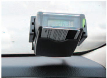
Figure 2. An ERP Gantry in Singapore

Source: Courtesy of Singapore land Transport Authority

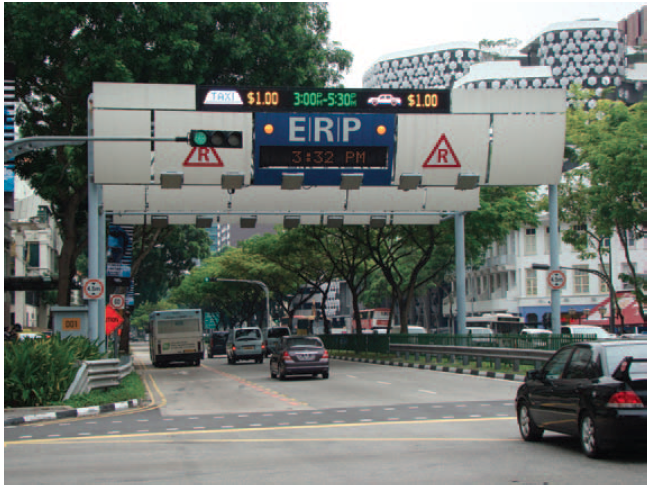
Figure 3. ERP Working Process

Resource: http://www.lta.gov.sg/content/ltaweb/en/roads-and-motoring/managing-traffic-and-congestion/electronic-road-pricing-erp.html

ERP Rates 

According to the Land Transport Authority (LTA), “ERP rates are determined by a quarterly review of traffic speeds of priced roads and during the June and December school holidays.” The LTA concluded that the prices are charged mainly based on two parts: Passenger Car Unit (PCU) equivalent and the time entering RZ. (See Table 2) Besides, the motorists should control their speeds between 20km/h to 30km/h on selected ways and between 45km/h and 65km/h on expressways.

Table 2.Two parts of Charges

Resource: http://www.lta.gov.sg/content/ltaweb/en/roads-and-motoring/managing-traffic-and-congestion/electronic-road-pricing-erp.html

We can see that the ERP rates vary for different time and roads periods and can be adjusted based on local traffic conditions. From Figure 3 we can see that 9 Am is an expensive time to drive, but in noon the rate is very cheap. For some alternative routs, the motorists don’t need to pay any fees. Therefore, this scheme encourages the motorists to make adjustments on their mode of transport, time of travel and travel route. The ERP scheme is very flexible and adaptive. However, some problems appeared. For example, to avoid higher charges time, some motorists would wait until the cheaper period started. To solve this problem the LTA introduced graduated ERP rates, which introduced a new rate for the last five minutes if the next period has a lower ERP rate.

Figure 3. EPR Rates and ALS Rates

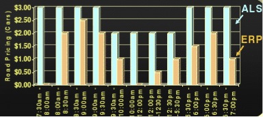
Resource: http://www.ibtta.org/files/PDFs/Chin_Kian%20Keong.pdf

The effectiveness of ERP

1) Traffic Impact

After replacing the ALS with ERP system, traffic levels have decreased a further 15 percent. In Figure 6, the traffic volume into the Central Business District (CBD) showed a significant decrease from 1975. Although the vehicle population and car population had been increasing, the traffic volume almost stayed unchanged and also showed a small decrease. In Singapore, increasing number of citizens chooses public vehicles as their main transportation tool, round 63% by public transportation.

Figure 6. Traffic Volume Changes

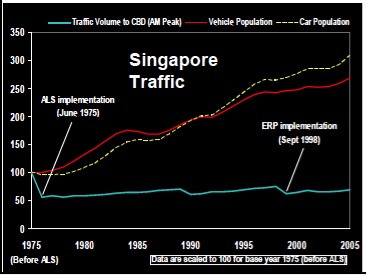
Resource: http://www.ibtta.org/files/PDFs/Chin_Kian%20Keong.pdf

2) Costs and Revenue

From Figure 5, we can conclude that compared with other countries, Singapore had very high ratio of annual cost to revenue, which results from high purchase and installation cost of ERP equipment and UI. However, the operating cost was very low. Singapore’s ERP system is operated by the control center Compared with other countries’ scheme, the ERP system is flexible and not labor intensive. As Walker (2011) showed, “the cost of managing and maintaining the ERP system has increased over the years, consistent with the increase in the number of gantries and IU numbers, but remains at 20–30% of total revenue collected, the objective is traffic management, not revenue generation.” For example, between 2007 and 2009, ERP revenue increased by $44 million, but at the same time, the additional registration fee (ARF) and vehicle tax revenue fell by $329 million in total. The revenue from the system is mainly used for construction and maintenance of roads and public transportation.

Figure 5. Cost-Effectiveness Matters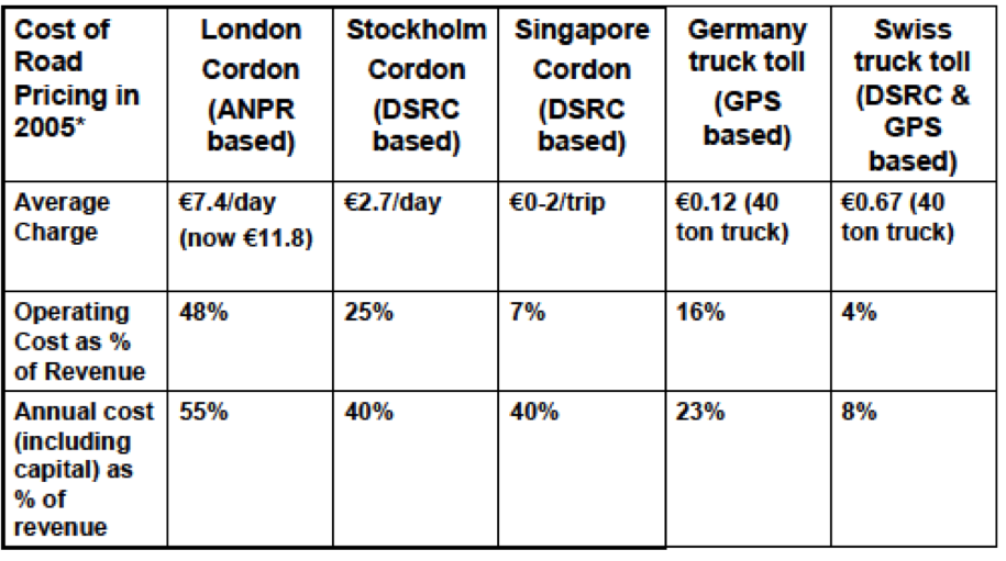

Source: European Conference on Transport Minister, 2006, http://www.cemt.org/topics/taxs/Paris06/Conclusions.pdf

Conclusion

In Singapore, technology has brought a lot benefits to the society. I think ERP is a very effective road management tool, which could be a lesson for other countries. The revenue neutral of this scheme avoid the fight from citizens. The motorists can enjoy a smoother drive, change their schedule to pay lesser charges and choose an alternative road. When we analyze the benefits of a road pricing scheme, we should think about externalities such as time saving, higher speeds, CO2 reduction, Fuel saving and also alternative road’s congestion problem. In my blog, I cannot get enough information on this point. In London’s case, we can have more sense of how to measure the efficiency of a road policy. 

References:

Land Transport Authority http://www.lta.gov.sg/content/ltaweb/en/roads-and-motoring/managing-traffic-and-congestion/electronic-road-pricing-erp.html

http://en.wikipedia.org/wiki/Road_pricing#cite_note-34

John Walker(2011), The Acceptability of Road Pricing http://www.racfoundation.org/assets/rac_foundation/content/downloadables/the%20acceptability%20of%20road%20pricing%20-%20walker%20-%20main%20report%20(may%2011).pdf

ERP System in Singapore http://duniainformation.blogspot.ca/2012/11/erp-system-in-singapore.html

http://www.imprint-eu.org/public/Papers/IMPRINT3_chin.pdf

http://ops.fhwa.dot.gov/publications/fhwahop08047/02summ.htm

http://www.cemt.org/topics/taxs/Paris06/Conclusions.pdf

http://www.ibtta.org/files/PDFs/Chin_Kian%20Keong.pdf

http://www.dac.dk/en/dac-cities/sustainable-cities-2/all-cases/transport/singapore-the-worlds-first-digital-congestion-charging-system/?bbredirect=true

Background

The Netherlands has the highest environmental taxes in the world. Citizens and companies in the Netherlands pay 27 billion euros annually, together with charges on polluting behavior. Water has always played an important part in Dutch life. The Netherlands(41,000 km2, including 3,000 km2 of fresh water and 4,000 km2 of saltwater) is a low-lying country in the delta of four European rivers: the Rhine,the Meuse, the Scheldt and the Ems. Since 1960, the quality of surface water in Netherlands deteriorated rapidly, which lead to government’s great concern. In the late 1960s the water boards were reorganized and they were provided with the responsibility of collecting levies for discharges. The rejection to proposal for large-scale state subsidies to the Water Boards for the construction of local sewage treatment plans results in “a full-recovery scheme based on revenues from emission charges  (in accordance with the polluter-pay principle)” (UCD). In 1970, the Dutch wastewater levy was set up with the 1970 Surface Waters Pollution Act and came into effect in 1971. Therefore the original aim for the state water levy is to curb water pollutions by using revenue to support municipal sewage treatment plan as well as in-house pollution abatement in industry.  Since 1996, the subsidy scheme for industry was abolished.

Coverage and Tax Rates

The levy is imposed on all direct and indirect surface water to surface waters. The tax rate varies for different polluters. Households pay a flat rate, small firms pay a fixed rate, medium sized firms and large firms can pay according to direct measurements. Here the medium sized firms also can pay by non-measured factors. I think if the households pay a flat rate, will this cause the distribution problem? Because the poor people maybe get worse off.  But until now I cannot find evidence on it.

The waste tax taxes the amount of waste that is delivered at a waste-processing firm or dumping ground (this tax is levied on the weight of the waste). The waste water tax applies to the discharges of organic material, mercury, cadmium, copper, zinc, lead nickel, chromium and arsenic. Here taking the year of 2008 to 2009 as an example to show main emissions to water.

http://www.wavespartnership.org/waves/sites/waves/files/images/Netherlands%20env%20accts%202010.pdf

The tax rates have increased many times since it was introduced. According to UCD, “from 1972 to 1990, the levy rate tripled and from 1990 to the end of the 1990’s the levy rate doubled once again”. The tax rate varies ate state level and at Water Boards level (regional level), it is 25 Euro per pollution unit for state waters levy and 37 Euro per pollution (on average) for Water Board levy. State waters are defined as the main rivers as well as the North Sea and are admonished by the water management department of the Ministry for Transport and Public Works.  There are 27 regional Water Boards in Netherlands and they are responsible for regional waters and to their sewage treatment plants. These Water Boards are powered by provinces, but their levy is not bond to the law. I think this maybe a issue for Netherlands water pollution control policy.

 Revenue

The revenue from the state waters levy is used to support both municipal sewage treatment plants and industrial in-house pollution abatement. Revenue recycling was particularly important during the early years of the scheme, when several of the most polluting industries were assisted in implementing emission reduction measures (RIZA, 1995).

When the levies were first introduced, several thousand consumers took part in an organized boycott campaign against their payment, as the levies were seen as unjust and the Water Boards as illegitimate. Consumers didn’t recognized themselves as polluters. However, the cost to the Dutch household is relative lower because there was less need for investment in public sewage treatment capacity. And also, the results seemed very positive. Andersen (1994) the levy system encouraged technology innovation which were promoted by subsidies from the levy, so this tax policy worked comparatively more efficient than similar programs in neighbouring coutries. In the meantime, the cost of this policy cannot be ignored. According to published data, in 1995, water pollution control costs made up about 25 percent of total environmental costs and ranked as send largest after waste management. Because I cannot get more recent data on this topic, I am concerned about the update information may tell a different story from what I did research on Netherlands waste water tax. And also Data on the annually discharged amount of damage units as defined by the waste water tax law are not available.

Reference: 

http://www.dutchdailynews.com/environmental-taxes/

RIZA, 1995. Waste-Water Charge Schemes in the European Union. A report for the European commission, Office for Publication of the European Communities.

Environmental Taxes: Implementation and Environmental Effectiveness (Environmental issues Series No.1), European Environment Agency, Copenhagen 1996, pp59-60

http://ec.europa.eu/environment/enveco/taxation/pdf/ch7_waste_water.pdf

On July 1^st, 2008, the Canadian province of British Columbia (BC) enacted North America’s first broad-based carbon tax designed to reduce greenhouse gas emissions (GHG). To support understanding of carbon policy in British Columbia, I will introduce some background and contextual information on carbon policy first.

1. The definition of GHG: 

GHG refers to the six greenhouse gases included under the international Kyoto Protocol carbon dioxide, methane, nitrous oxide, nitrogen triflouride, sulphur hexafluoride, hydrofluorocarbons and perfluorocarbons.

2.  Carbon Policy: carbon tax and cap-and-trade.

1) Carbon Tax is more about ‘Price’. According to BC Ministry of Environment, ‘the carbon tax puts a direct price on each tonne of carbon (or GHG emitted) thereby sending a price signal that will, over time, elicit a market response across the economy to reduce carbon emissions.

2) Carbon cap and trade system is more about ‘Quantity’. According to BC Ministry of Environment, the carbon cap system sets an absolute limit on the quantity of carbon emissions across specified industrial sectors. At the same time, the permits for each tonne of carbon emissions that specified industrial sectors get can be sold and transferred within the system.

Based on the environmental economic models we learned before, the below diagram can provide a clear picture of how does the carbon policy work.

A Model with A Single Polluting Firm
Consider a polluting firm that facts an increasing marginal pollution abatement cost curve. The benefit-cost analysis has determined that optimal abatement occurs at e* where the marginal benefit and marginal cost curves intersect.
Carbon Policy–Tax:
If carbon abatement < e*, the tax bill (A+B) > the marginal abatement cost bill (B), the firm will choose to abate instead of paying the tax.
If carbon abatement >e*, the tax bill (D)< the marginal abatement cost bill (C+D), the firm will choose to pay the tax and continue to pollute. In this situation, the abatement cost to this pollution firm=B+C+D and the government can get tax revenue=D
Carbon Policy–Carbon Cap:
The abatement cost to the pollution firm=B and government cannot get revenue.

A Model with Two Polluting Firms
The two-panel diagram illustrates two different increasing marginal abatement costs. The intersection of the two marginal abatement costs is where economic efficiency achieved. (“equimarginal principle).
Carbon Policy–Carbon Tax:
To abate the emissions to e*, the highest cost firm: tax bill(B+C+F+G) and abatement costs(K)
the low cost firm: tax bill(C+G) and abatement costs(J+K)
Carbon Policy–Carbon Cap-and-Trade:
A carbon cap is set by issuing carbon permits to polluting firms. The abatement cost to the low abatement cost firm=C and to the high abatement cost firm=D+F+G+K. We can suppose that the blue line is a a demand curve for permits and the green line is a supply curve for permits. Trading will reduce overall abatement costs by area D+F. And in this policy, the abatement cost to the pollution firms equals to that of tax policy, is C+G+K

The carbon tax and carbon cap-and-trade can achieve the same level of efficiency by achieving the optimal abatement level at the minimum cost. But the distributional implications are different, the firm can lower the cost through carbon cap-and-trade and the government can get tax tax revenue with a carbon tax. Form the second model, we know that the carbon policy can encourage the firms to adopt new technology to lower the marginal abatement cost.

The above analysis shows the theoretical side of carbon policy, now we will look at the real-life example of implementing carbon pricing policy in BC, Canada in the following paragraphs.

A. Carbon Tax:  B.C. carbon tax costs increase at a rate of $5 per tonne of CO2 emitted per year from the initial level of $10 per tonne in 2008 up to $30 per tonne in 2012. the carbon tax is applied indiscriminately across industrial sectors and households solely based on the carbon intensity of the fuel type, which means the taxpayers pay the same on every unit of emission.

Problem:The carbon tax can lead to an increase in fuel price. Because BC has among the highest levels of poverty and inequality in Canada, a pressing concern is the potential for unfair impacts of carbon pricing on the poorest.. It is easy for the rich people to make adjustment on their consumption proportion. However, it is hard for the poorer to adapt to.

BC Solution: The BC government’s policy of “revenue neutrality” requires all carbon tax revenues to be transferred back to British Columbians in the form of personal and corporate income tax cuts, and credits for low-income households.

<New problem>:  According to Marc Lee (2011) , ‘BC’s carbon tax regime has in fact been revenue negative—the value of tax cuts and credits has exceeded carbon tax revenues, primarily due to corporate income tax cuts.’ and also the low-income credit part is decreasing.

The distribution of the tax revenue return is not appropriate, because most of the revenue are transferred to corporate income tax cuts in the future. That means the policy of revenue neutrality cannot achieve the goal of lowering the negative affect on low-income household or person. This will result in poorest’s resistance to this policy.

B. Carbon Cap-and-Trade:  B.C. is working with the Western Climate Initiative (WCI) partner jurisdictions to create a regional carbon market across a diverse set of emission sources.

Problem: The larger the carbon market, the greater the range of emission reduction opportunities available to emitters and the lower the cost of compliance. However, I think this market is not very stable and cannot work very well, there are many jurisdictions joint at the beginning, but many quit already.

Here is the detailed information on carbon policy Coverage:

In B.C., “downstream” combustion of gasoline, diesel, marine and aviation fuels and residential, commercial and industrial (below the cap and trade compliance threshold) use of natural gas, propane and home heating oil would not fall under the cap and trade program as they would continue to be subject to the province’s carbon tax.

The BC carbon tax covers about 73% of domestic GHG emissions and the remaining 27% come from non-combustion sources including industrial processes. I think the coverage should be extended in the future.

In all words, I think BC are trying to make comprehensive carbon pricing policy to control the GHG emissions by making creative policy. I appreciate this action. At the same time, I think there are always some gaps between plan and reality. When applying this policy to really life, the externality of this policy should be considered, especially from disadvantaged groups’ side.

References:

http://www.ldlc.on.ca/uploads/2/7/8/8/2788943/ccpa-bc_fair_effective_carbon_full_2.pdf

http://www.env.gov.bc.ca/cas/mitigation/ggrcta/pdf/carbon-pricing-bg.pdf

http://www.fin.gov.bc.ca/tbs/tp/climate/carbon_tax.htm

http://www.env-econ.net/carbon_tax_vs_capandtrade.html

Through this blog, I plan to add more information on Fisheries’ model. I feel that our prof. spent more time on this topic. I believe that it worth learning more information about it.

I want to start from the basic concepts.

Maybe because I am an international student, when I heard the work ‘Fish Stock”, I understood it as fishers stock fish. However, Here ‘Fish Stock ‘ could be interpreted as a population of a fish species that lives and is able to reproduce itself within a given geographical.

There are many factors can affect the fish stock. Based on what I learned from a journal, recruitment, natural mortality, individual growth and harvesting can lead to changes in fish stock. The formula can be represented as follows:

Stock change=Recruitment+ Individual growth-Natural mortality-Harvest. There are several inputs a fishing harvest firm should invest in such as fuel, bait, gear and labor. In our lecture we use effort as the fishing input.

In the following part, I will introduce two concepts: MSY (Maximum Sustainable Yield) and MEY (Maximum Economic Yeild). And also the diagrams below show short-run harvest for five different effort levels. For the smallest effort E1 the harvest curve crosses the growth curve for stock level X1 and harvest H1. Thus, a small effort – over a sufficiently long time to let the stock reach equilibrium – gives a high stock level and a relatively small catch. The same trick happened on E4 and E2. We can see that the highest possible harvest is reached for effort level E3 and this harvest is called MSY (maximum sustainable yield).

The stock-level & growth rate curve can be transformed into a sustainable harvest effort curve.Resource rent can be translated as the difference between total revenue and total cost for each effort level. This level can be achieved through MC=MR. The positive difference are maximized. At the same time we can find MEY(Maximum Economic yield).

What I went right?

Last week, I was busy preparing a presentation for another course, therefore I didn’t spare time for my blog. At the same time, I missed the opportunity of latest released report. Unfortunately, I went six long positions, which resulted in a big loss and I couldn’t get out of this bad situation. Until now, I am still looking forward to another chance to gain my money back.

On Nov. 9^th, 2012, USDA released the supply & demand report on three commodities: soybeans, corn and wheat. According to this report, US soybean production was 80 million above trade expectations and “ the jump in world ending stocks is a significant concern. As for corn, USDA pegged 2012/13 corn production at 10.725 billion bushels which was 91 million above expectations. However, all world wheat production was experiencing a downward trend, about 1.5 million from the October estimate. However, wheat and soybean are substitutes, the same trend for these days are common.

Daily Price Change

 The Road Ahead:

These days I For next week, I will focus on how to use technical analysis to forecast price. The technical analyst focuses purely on market information, but also volume and open interest figures.

Soybean:

From this chart, we can see that from August to now, there is a sign of inversed head and shoulder (Top). This involved three phases-the formation of the left shoulder, the head, the right shoulder. Therefore, I think there will be a upward trend in Nov. 14^th contract.

                         Left shoulder              Head Right                     shoulder

And also the above analysis can be confirmed by moving average analysis. Here are three moving average lines, which based on different year range. The most basic way to trade using just the moving average is to buy when the price of a commodity breaks above the moving average line.

Corn:

In recent days, the corn price fluctuates a lot. I cannot find any specific signs for future trend. Therefore it is hard to predict. Based on the former experience, in October, there was a similar slump and then back to the former level and then stayed stable for a while. Therefore I guess in the next few days, there will be an increase in price.

Wheat:

As for wheat, the price reached to the top in Nov and then showed a downward trend. At the same time, the open interest and volume is relatively high when compared with last few months, which shows a strength behind the downward trend. Therefore I think the July, 2014 trend will continue.

And from the moving average lines, we can see that the price of the moving average breaks below the moving average line, so sell the contract.

References:

http://www.agrimoney.com/futures.php?page=chart&sym=ZCN14

http://futures.tradingcharts.com

Cool Resources:

Cool Resources:

http://www.forexpros.com

This website is really cool for finding commodities news, charts, technical analysis and so on. Especially this website has weekly outlook of Grain futures, which can give you some information on how to move on for next week.

I am looking forward to more feasible resource to help me with my technical analysis.

The Road Ahead

About Exchange Rate:

Last week, I got some suggestions from Araza, he asked me whether exchange rate has a significant effect on world price of crops. Therefore this week I have a look at it.

A stronger US dollar reduces the competitiveness of dollar-denominated exports such as many commodities by making them less affordable to buyers in other currencies. Therefore the demand of consumers from exporting countries will be less, which would increase the price of crops. According to Agrimoney.co, Chicago’s November soybeans fell 2.0% to $15.27 a bushel, with the better-traded January contract showing a 2.2% fall to $15.26 ¾ a bushel. At the same time, December corn fell by 1.4% to 7.39 ½ a bushel, while December wheat eased 0.2%, to $8.64 ½ a bushel.

About Production prospects:

1. Weather: The worst crop conditions have forced some farmers to reseed the wheat, which reveals a worst start since records began.

In other areas, the downgrades follow a further period of weather extremes, following last season’s drought, which has landed much of Argentina and southern Brazil with excessive rain, while leaving many central and northern parts of Brazil with too little moisture.

The heavy rainfall delayed plantings of soybeans with data showing that farmers have planted only 3.6% of expected hectares. This situation also happened on corn seedings.

1. Policy: Russia decided to remain open to grain exports despite a poor harvest this year. First, it means that the country may have some more supplies to ship this season. Secondly, this policy encourages Russian farmers to raise sowings of winter crops and spend more on the crop. Russia is propping up domestic supplies, and keeping prices somewhat in check, by releasing grain from state reserves.

Conversely, in Ukraine farmers will likely reduce winter plantings, because of the uncertainty sown by official statements on curbs, culminating last week in the country’s farm minister confirming a ban while the prime minister’s office denied a decision had been made.

Based on above analysis, the price of wheat is hard to estimate. I think the above information is not enough for me to make my guess. Therefore, I will follow Andrew’s step to learn some basics of technical analysis. Besides, this week I will pay attention to the report release date:

1. Supply and Demand Report will be release on Nov. 8^th
2. The USDA was scheduled to release its updated crop estimates on November 9^th

And According to the data from Forexpros.com, “market players should focus on the USDA’s weekly crop progress report on Monday as well as Thursday’s weekly exports data and Friday’s updated Supply and Demand Report.”

References:

http://www.agrimoney.com/feature/ag-investors-brace-for-controversy-as-us-stocks-data-loom–170.html

http://www.forexpros.com/news/commodities-news/grain-futures—weekly-outlook:-november-5—9-240264

What I went right?

For this week, based on my last week’s analysis. The tight wheat stocks of major exports and the negative prospect of corn will lead to a higher price. Therefore I chose long positions on future contact of wheat and corn. At first I got the knowledge that soybean productions will raise. However, I got some feedbacks of my blog from Vicky and Araza. They suggested me to do some other researches such as exchange rates and acknowledged me that China as one of biggest exporter of soybeans will increase its imports. Therefore I changed my choice. The depreciation of US currency would encourage other countries to import more crops, which create more demand. Therefore I bought a 2014 July contract on soybeans. Here are my trading information and daily price change of crops.

Daily Price Change

1. What I went right?

For this week, based on my last week’s analysis. I planed to use spread to earn more. In the short run, the corn price was decreasing, but in the future, the corn price would go up because of the shortage of stocks. Therefore I went a long position on July contract in 2015 and a short position on March contact in 2013. The result was really pleasing. It seemed like I made a good choice. Although I lost some money on July contract, 2015, it shows an increase trend now. Here are my account information:

Daily Price Change

2. The Road Ahead

About future stocks:

According to the news from Agrimoney.com, inventories in major exporters such as Canada, the European Union and the US are forecast to be a 3m tones drop to 96m tones. Just as IGC said, “inventories for the major exports will be even tighter and the smallest for 17 years.” The following shows more information about the stocks situation.

 About Production prospects:

For corn, the production prospect was cut to below the USDA figure. It is also estimate that “northern hemisphere production prospects have mostly worsened.”

For wheat, “lower yields in the European Union and Kazakhstan, as well as deteriorating crop prospects in Argentina and Australia, reduce the forecast for world production to 655m tones,” the IGC said. At the same time, China increases imports of wheat. Chinese wheat imports look set to trounce market expectations for 2012-13, putting extra upward pressure on world prices. In Ukraine, a ban on exports of the grain will be executed from Nov. 15^th.
For soybean, the IGC was optimistic to soybean production, raising their world production estimate by 8m tones to 264m tones. The weather for southern American crops plays a very key role in world soybean production.

Based on above analysis, I would go with long positions on corn and wheat, especially on 2014 or 2015 contract and a short position on soybean.

References:

http://www.agrimoney.com/news/surge-in-chinese-wheat-imports-to-set-a-trend–5139.html

http://www.agrimoney.com/news/top-exporters-grain-stocks-to-fall-to-17-year-low–5147.html

 3. Cool resources

http://www.dtnprogressivefarmer.com/dtnag/home

I got this cool resource from Sean, it is a website focusing on farmers.There are a lot cool information here such as news, market, livestocks, farm business and etc. Especially, this website include many farmers’  blogs .They blog from various perspectives such as market matters, technically speaking, ethanol blogs, production blogs, policy and so on. I think this is amazing.  These farmers or blogers have their own predication about the market from different viewpoint. I think this will be very helpful for us to get more information.

2. The Road Ahead

Before the next report releases on November 8th, I think the price change of crops will be hard to predict. Therefore the short-term downward trend may change very rapidly. The weather change would contribute to the supply analysis in the next year.

According to what Telvent DTN Inc. said in a report yesterday, showers forecast for the soybean- and corn-growing areas in Brazil this week will be mostly light and temperatures will remain above normal after dry weather depleted soil moisture, therefore the crop stress may return to Brazil.

Also in Argentina, the largest soybean shipper behind Brazil and the U.S., heavy rains this month may delay planting, and also affect corn and other winter crops.

According to the recent October report on cereal supply and demand brief, a decline in world cereal production in 2012 from the record in 2011. The decrease will result in a significant reduction in world inventories by the close of seasons in 2013 even with world demand sliding as a result of high prices.

So far, based on the above information, I would still hold a short position on the future contract in 2012 and long position on 2014 or 2015’s future contact. We will see what will happen. I will pay attention to the next report coming on November 8th. I think I will take advantage of the release date.

References:

http://www.fao.org/worldfoodsituation/wfs-home/csdb/en/

http://www.bloomberg.com/news/2012-10-24/soybeans-climb-on-concern-crop-stress-may-develop-in-brazil.html