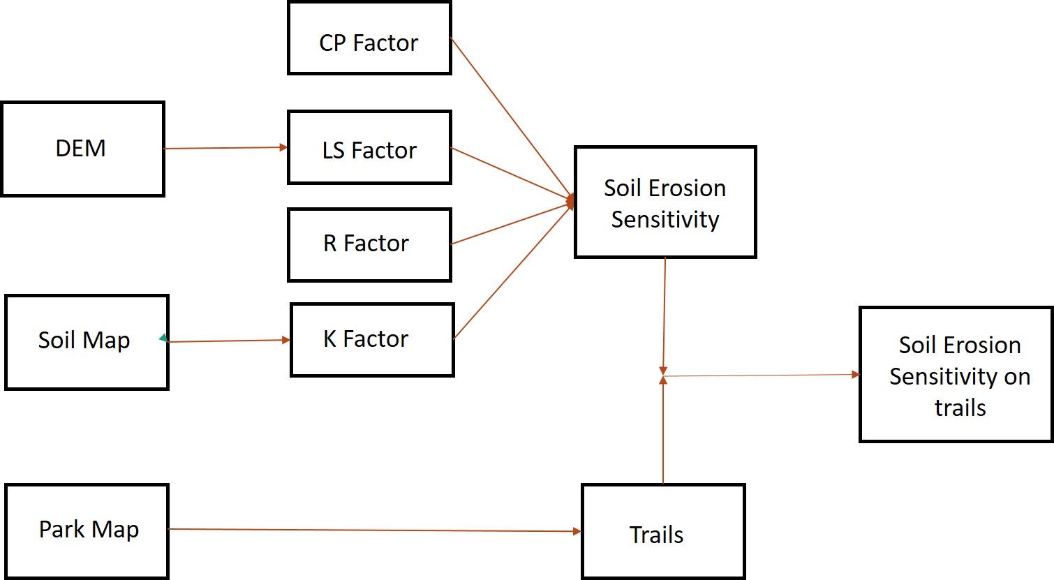
Figure 4: Steps to calculating soil sensitivity on trails using RUSLE
In order to model soil erosion at cypress, the RUSLE model was used. RUSLE stands for Revised Universal Soil Loss Equation and is the stand equation to model soil erosion. This revised form of the equation allows to model high gradient slopes that can be seen at Cypress. The equation:
Soil Erosion( A) = LS x K x R x C x P
Where:
LS Factor: length (L) and slope steepness (S) factor
The factor represent the effects of slope length and slope steepness on the erosion of a slope. The combination of the two factors is called the “topgraphic factor.” The L factor is the ratio of the actual horizontal slope length to the experimentally measured slope length of 22.1-m. The S factor is the ratio of the actual slope to an experimental slope of 9%. The L and S factors are designed such that they are one when the actual slope length is 22.1 and the actual slope is 9%.
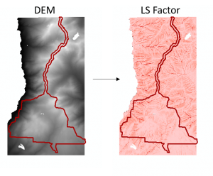
Figure 5: DEM with black being low elevation values converted to the LS factor where dark red are the areas with highest LS values. The maroon is the park boundary
A DEM with resolution of 25mx25m was clipped using Park outline. The DEM was then made to be Sink free. Slope, Flow direction and Flow accumulation layers were calculated and finally the LS factor layer was created using map algebra with the following equation (Pelton et. al. 2015):
Power(“flowacc”*[cell res ]/22.1,0.4)*Power(Sin(“sloperasterdeg”*0.01745)/0.09, 1.4)*1.4
Where: “flowacc” = Flow accumulation raster, [cell res] = Resolution of DEM in meters, “sloprasterdeg” = Slope Raster in Degrees
K Factor: Soil Erodibility factor in t h MJ-1 mm-1
Soil map was clipped using DEM outline. Each polygon in soil map is a survey area with details about the types and percentage (%) of soil present within survey polygon and the % of silt, clay, sand, organic matter etc. The K factor for each soil present in polygon was calculated using following equation from (Wischmeier and Smith 1978):
K= [2.1 x 10-4 x (12 – a) x [Ss x (100 –Sc)) 1.14 + 3.25 x (b – 2) + 2.5 x (c – 3)] /100 x 0.1317
Where Ss and Sc are the products of the dominant size component, and the percentage of the clay, respectively. a is the percentage of organic matter in %, b the soil structure (Table 3 in Fig 6), c the soil saturation capability (Table 4 in Fig 6).
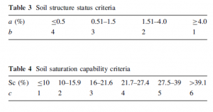
Figure 6: Tables used to determine values of b and c factor ( Chen 2011)
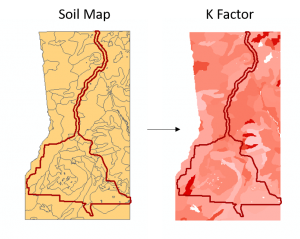
Figure 7: Soil map with all the survey polygons being converted to map with the K factors. Dark red indicated higher K factors
K factor for each soil was weighed to the % of soil present in the polygon- giving a weighted K factor for each survey polygon. The layer was then converted to raster.
R Factor: Rainfall Erosivity factor in MJ mm ha-1 h-1 ya-1
Calculated using the following equation:
R= 0.1281 x I30B x P – 0.1575 x I30B
Where I30B is 30 mins intensity (mm/h), P is annual rainfall (mm) (Chen 2011). This data was calculated using a Metrovancouver report
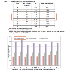
Figure 8: Table showing data chosen to get the R factor (Metro vancouver)
CP Factor: Cover (C) and Conservation Practices (P) factor
Given the value of 1 since there is no cover on trails (Tomczye 2011)
Trails
The trails came from a trail map (Figure 9). The Map was georeferenced and then traced on to form a polyline layer.
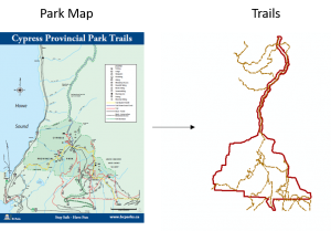
Figure 9: Trails and park boundary traced using park map
Soil Sensitivity on Trails
The factors were multiplied using map algebra to give a raster output with the soil erosion sensitivity of the area. This was then converted to a point layer. This layer was clipped using the Trails polyline layer to give soil erosion sensitivity on trails. The results of the three layers are given on the results page.