1. Preliminary Research – criteria determination (Factors/Constraints)
Looking for new affordable housing locations is a multiple criteria evaluation(MCE) that take into account what is necessary to consider when building them. The very first step of this project, therefore, is to research on, and reference to the current corresponding governmental regulations and guidelines.
City of Toronto Council endorsed the Housing Opportunities Toronto (HOT) Action Plan 2010-2020 as a road map to steer the work and investment decisions of the City of Toronto as they relate to affordable housing in partnership with federal and provincial governments over this decade2 . This project, therefore, consults on HOT Action Plan 2010-2020 to identify the relevant criteria (factors and constraints) of building affordable houses.
It is important to know that the Plan is aligned with, and complementary to, other key city initiatives, including Official Plan, Transit City, and the Change is in the Air climate change strategy. It builds on and supports several other long-term goals such as the revitalization plans of Toronto Community Housing and the Prosperity Agenda’s goal to position Toronto as a leading 21st century global city by encouraging business investment, stimulating the economy, attracting key workers and creating opportunity and livability for all residents. Therefore, affordable housing should power economic prosperity, a greener city (E&S), livable neighbourhoods and healthy people.
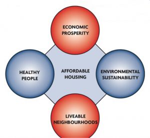
Core criteria of building affordable housing (Based on Housing Opportunities Toronto Action Plan 2010-2020)
|
Themes |
Regulations from Action Plan 2010-2020 |
Corresponding criteria for this project |
|
Economic prosperity |
a) Attracting key workers, a skilled labour force and immigrants b) Encourages businesses to locate and expand locally c) Costing less on average ($23 per day) than use of emergency shelters ($69), jails ($142) and hospitals ($665) when people are homeless |
1. Affordable houses should locate in economically active area; avoid building in residential/recreational/ governmental & institutional area/waterbody2. Low friction values (costs) area is preferred |
|
Environment and sustainability |
a) Allows people to live closer to where they work, reducing vehicle-related greenhouse emission | Locate affordable houses where have convenient and accessible access to transportation – Subway Stations |
|
Livable neighbourhoods |
a) Makes streets safer and encourages business and other investments in neighbourhoods b) Reducing concentration of poverty, improves health, safety and quality of life for residents c) Diverse neighbourhoods provide opportunity and affordability in all 44 wards across the City |
Locate affordable houses where are relatively safe – city crime rate |
|
Healthy people |
a) Increase stability and security results in better mental and physical health b) Improve educational outcomes and opportunities for children |
Affordable houses should locate in areas with a variety of amenities – mental service / hospitals / educational institutions |
It is important to realize the unique confidentiality characteristics of location data and limited, non-public data access present special challenges for geospatial research and its societal applications. This project, therefore, will mainly focus on 7 factors (Educational Institutions / Subway Stations / Hospitals / Mental Service Centers / Skill Training Centers / Crime Rate / Low-income Group Distribution) and 2 constraints (Zoning/current affordable housing sites) we are capable of accessing. It may inevitably affect the objectivity of research results. The corresponding discussion will be presented in the Limitation section.
2. Standardization of factors/constrains
We use Raster Calculator to normalize the values of each factors. To do that, we build a Map Algebra expression that transforms different measuring values from the factors to a range of 0 to 1. In words the linear expression will be:
1- ( (factor – Minimum value of (factor) ) / (Maximum value of (factor) – Minimum value of (factor) ) )
We apply this expression to each of the factors to convert them into a common scale.
3. Determine the weights using MaxEnt
MaxEnt is a stand-alone Java application for modelling species niches and distributions by applying a machine-learning technique called maximum entropy modelling. From a set of environmental grids and geo-referenced occurrence localities, the model expresses a probability distribution where each grid cell has a predicted suitability of conditions for the species. We are inspired by its function and therefore apply it into our project. Maxent can not only discovers significant results of each variable’s weighted distribution for the factors, but generate a picture which presents a MaxEnt model predicted condition.
To perform a run, we need to input a file containing presence localities as “samples” in .csv format, and a series of directory environmental layers in .ascii raster grids format. In our case, the existed affordable house locations are served as “samples” and the seven factors we identified are the environmental layers.
Technically, MaxEnt generates a probability distribution over pixels in the grid, starting from the uniform distribution and repeatedly improving the fit to the data. The gain is defined as the average log probability of the presence samples, minus a constant that makes the uniform distribution have zero gain. At the end of the run, the gain indicates how closely the model is concentrated around the presence samples. In our case, the run produces multiple output files, of which the most important for analyzing our model is an html file. The entire file is attached in the Results section.
4. Evaluation using MCE algorithms
As mentioned above, Maxent model is capable of determining the weighted distribution for each factor. Therefore, instead of using an analytical hierarchical approach to calculate the weights, we refer to the weights assigned by Maxent directly.
The following table gives estimates of relative contributions of the variables (the factors) to the Maxent model. To determine the first estimate, in each iteration of the training algorithm, the increase in regularized gain is added to the contribution of the corresponding variable or subtracted from it if the change to the absolute value of lambda is negative. For the second estimate, for each environmental variable, in turn, the values of that variable on training presence and background data are randomly permuted. The model is re-evaluated on the permuted data, and the resulting drop in training AUC is shown in the table, normalized to percentages. In the case of the project, we used the value from Permutation Importance as weights (as shown below):
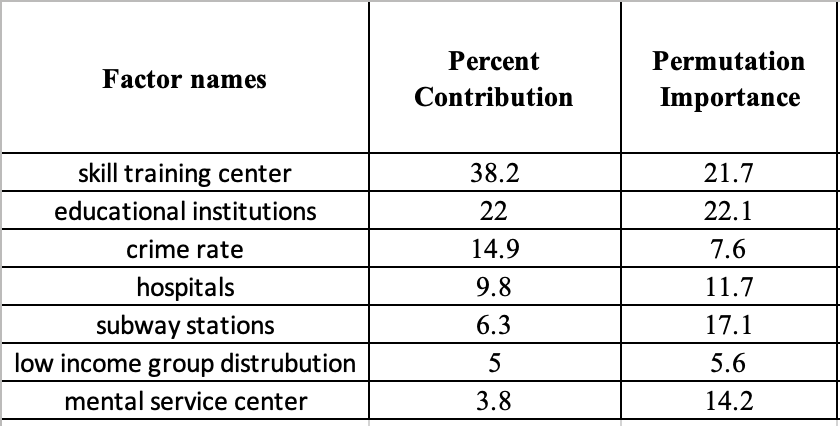
Relative contributions of the variables (the factors) — Analyzed by using Maxent model
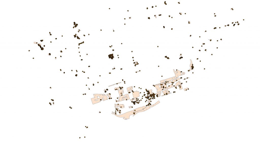
To conduct the actual weighted linear combination, we selected the sever factors’ rasters and then ensure that the appropriate weight, as determined in Maxent, is associated with each raster, and we used the Weighted Sum tool. The resulting raster has values that range from 0 to 1. We have set a goal to see which areas would be the most suitable for building affordable housing if we were to increase the number of affordable housing by an additional 10%. To set the class limits, we have reclassified our classes into applicable and non-applicable areas. In order to set the breaks between the two classes, we would need to find enough pixels that are 40 square meters (40m x 40m) per pixel to represent the total area of that additional 10 % affordable housing. In addition, we would need to know the average area of a single affordable housing in order to derive the area required since we don’t have a detailed report on the construction files of existing affordable housing. Instead, we have shapefile of current affordable housing including their geographic coordinates and current zoning categories that are made up of polygons. We did join based on spatial location after setting both layers to the same projection for accuracy purpose. Afterwards, we used the combined layers of Zoning categories and Current Affordable housing to find the polygons with a count of more than 0 housing in them. We can use select by attribute to export the layer only containing zoning of affordable housing and the statement is “Count_” > 0. The affordable housing that fall in those zoning is shown below:
![]()
Once we have exported our layer containing current affordable housing, we can use geometry calculator to summarize the total area for those polygons. Since we are only interested in the area for a single social housing so we divided by the total number of affordable housing.
The area of 10% of current affordable housing = Total area of current affordable housing in meters / Number of total existing affordable housing
Now we have the area of a single affordable housing then we can multiply by 10% of current affordable housing to determine the applicable area shown in results. The number of pixels (40m x 40m) used to select 10% of current affordable housing would also be used to be selected as a breakpoint between applicable area and non-applicable areas.
5. Sensitivity analysis
Similar to Lab2, we performed a sensitivity analysis to find out how variations in weights would affect the results. This is because the choice of weighting factors is somehow subjective, even though the weights is based on the MaxEnt results. To do so, we used the Model Builder to perform an equally-weighted analysis (each weight = 0.142) and then overlay the two sets of MCE results to see how they differ. The two models we used are presented below:
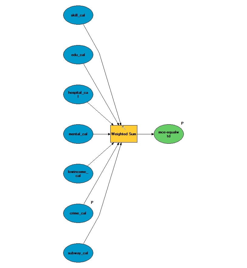
MCE using the equal weights
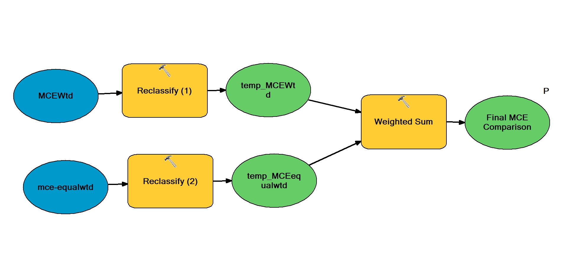
Overlay of the two MCE results
MCE Weighted (MCEwtd) only results show that there are area of 12.14km2 that is suitable for affordable housing, while MCE Equally Weighted (MCEequalwtd) only results shows area of 11.58km2. Area that both MCE Weighted and MCE Equally Weighted results overlaps have the total area of 6.91km2. This shows that using different weighting scheme will results in great changes that 43% of the optimal area will be at different location. The results of sensitivity analysis is shown below:
Please note that unless stated otherwise, projection for all maps is UTM NAD 1983 Zone 17
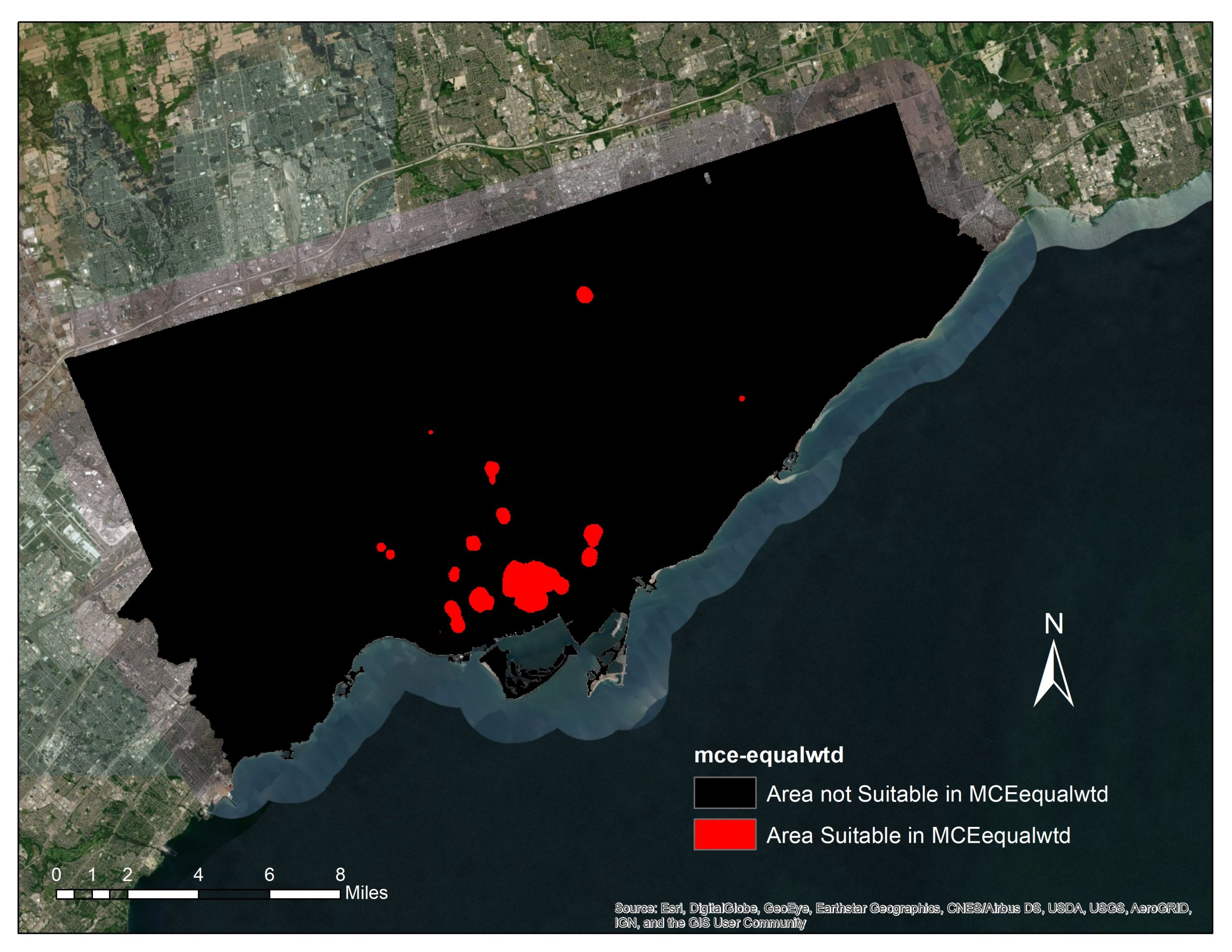
Results of MCE Equal Weighted
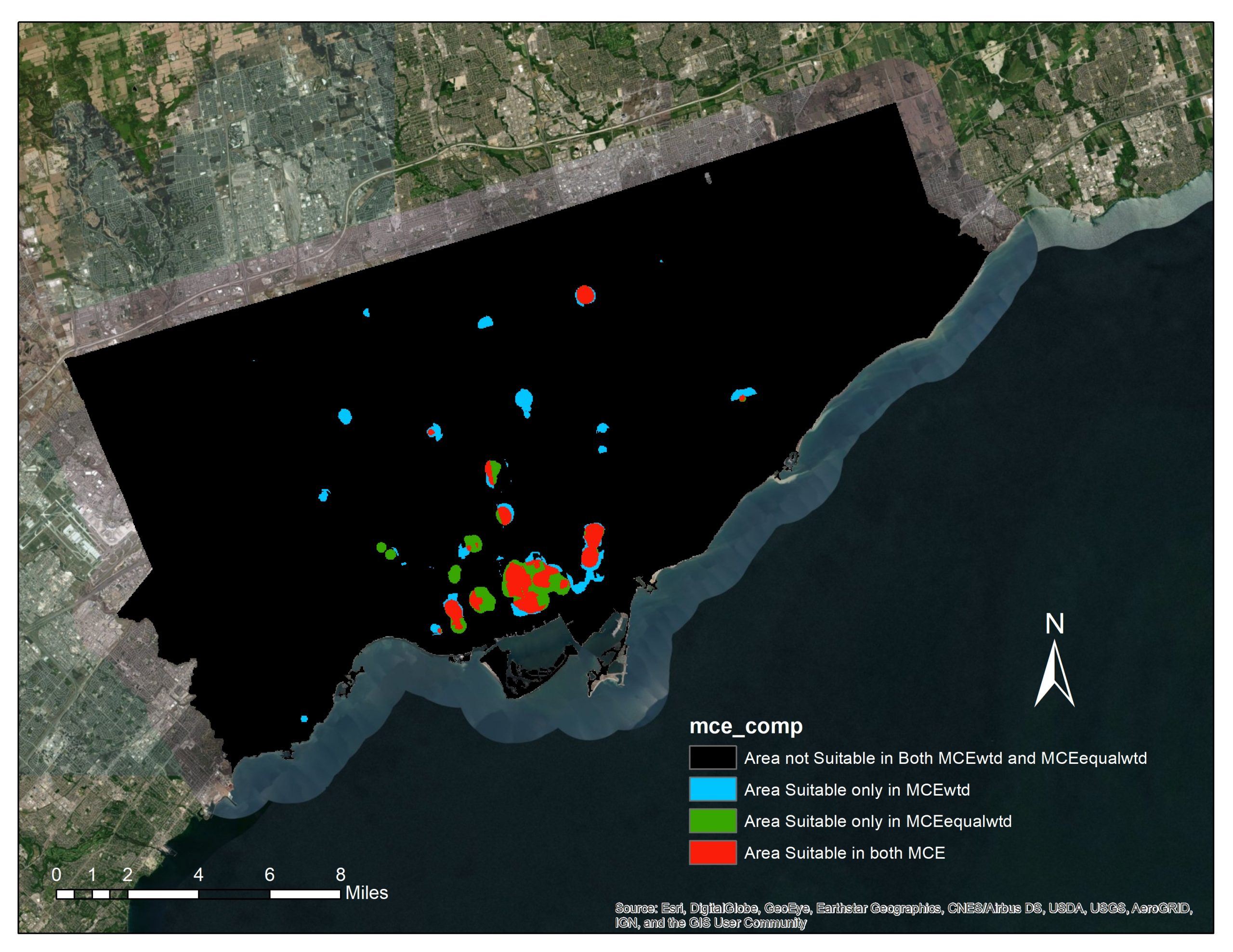
Results of Sensitivity Analysis
6.Apply the constraints
The final step of our MCE was adding constraints. As mentioned above, we identified specific zoning area and current affordable housing as constraints in MCE. Areas that are not suitable for affordable housing and should be excluded are buffer zone of the current affordable housing, open space, utilities & transportation institutional and residential area. We first performed “Select by Attribute” in the original zoning shapefile to extract all “constraint” area to one layer, then used raster calculator to add constraints to the previous MCE results. After adding constraints, 58.5% of the area in the original MCE results (12km2) are excluded, leaving only area of 4.97 km2.