
It’s incredibly difficult to assess the impact of an electoral reform ex ante. The problem is that parties’ and voters’ strategies are endogenous to the electoral system. This is one reason why the analysis of electoral reform so often has to operate on the basis of first principles. However, given the vagaries of social choice theory (generally no equilibrium for 3+ options in 2+ issue dimensions), there are limits to what we can say on the basis of first principles. For this reason, it’s still useful (and interesting) to look at data to learn about the impact of electoral reform.
The Spaniel is on record as preferring a “ranked ballot” electoral system – or the “Alternative Vote” (AV) as the system is known in Australia, where it has long been used at federal and state elections.[1] With their majority, the Liberals can impose an AV on the country – and, as I have argued previously, they have strong incentives to do so. Theoretically, AV works to the advantage of large, centrist parties like the Liberals. Correspondingly, it (theoretically) works to the disadvantage of both smaller parties and identifiably left- or right-wing parties; the former are disadvantaged by AV’s use of single-member districts; the latter, by the fact that they are less likely to be the second-preference of many voters.
Given that, it is interesting to look at how AV has worked out Australia, how the transition from FPTP to AV in Australia altered the effective number of parties that contested elections and won seats, the proportionality between votes & seats, the support for third-parties, and the level of electoral volatility. (Keep in mind that electoral reform was itself often undertaken by incumbent government’s in response to a threatening change in the party system, e.g., a growing Labor party.)
The Australian experience with AV is quite unique; I know of no other major country that has had such long experience with AV. But that makes it problematic to draw inferences about how AV might affect Canadian politics: we can’t know which aspects of Australian electoral and party competition are due to the inherent dynamics of AV and which are due to Australia being, well, Australia. To get around this (but, to be honest, only part way around this), I examine elections in Australia’s five mainland states as well as in the Commonwealth.[2] To the extent that trends are common across all 5 states and the Commonwealth, we can assume that that’s due to the (common) electoral system and not the peculiarities of the state.
The Australian state data are especially useful because, like the Commonwealth, the five mainland states used FPTP before adopting AV. This allows one to assess the impact of transitioning from FPTP to AV within each state. Now, the transition was not always direct as Table 1 below shows: NSW experimented with a two-round plurality system (of the sort used for elections to the French National Assembly), STV, and the Contingent Vote before adopting AV; Queensland only adopted AV in 1963.[3] In addition, FPTP was not always employed with single-member districts. South Australia applied both the plurality rule and the alternative vote in 2- and 3-seat districts.
Table 1. Electoral Systems used in Australia, 1890-2015
|
C-W |
NSW |
QLD |
SA |
VIC |
WA |
|
| FPTP |
1903-17 |
1891-1907 |
1941-60 |
1893-1927 |
1892-1908 |
1890-1905 |
| 2-RND |
1910-17 |
|||||
| STV |
1920-25 |
|||||
| CV |
1927 |
1893-1941 |
||||
| AV |
1919- |
1963- |
1930- |
1911- |
1908- |
The Effective Number of Parties
One of the first things a political scientist likes to know about a country is how many parties contest elections and win seats. The longstanding notion is that the number of parties is closely related to political stability, the potential for polarization, and the capacity of electoral politics to represent diverse interests. Now, not every party counts as interesting or relevant; for example, we probably want to discount fringe parties that obtain .5% of the vote — but arbitrarily ignoring some parties (which ones?) is problematic. Consequently, political scientists tend to focus on the effective number of parties (Laakso & Taagepera 1979). We either count the effective number of electoral parties (i.e., the number that contest elections) and/or the effective number of legislative parties (i.e., the number that win parliamentary seats). We obtain the effective number of electoral parties by constructing a Herfindahl-Hirschman Index (HHI) of parties’ vote shares, with vote shares expressed as proportions. Similarly, we obtain the effective number of legislative parties by constructing a HHI of parties’ seat shares, with seat shares expressed as proportions. (The difference between the two statistics can be informative. For example, we often see large deficits in the number of parties that contest elections and win seats in transitional democracies where expectations about parties’ competitiveness have not yet congealed.)
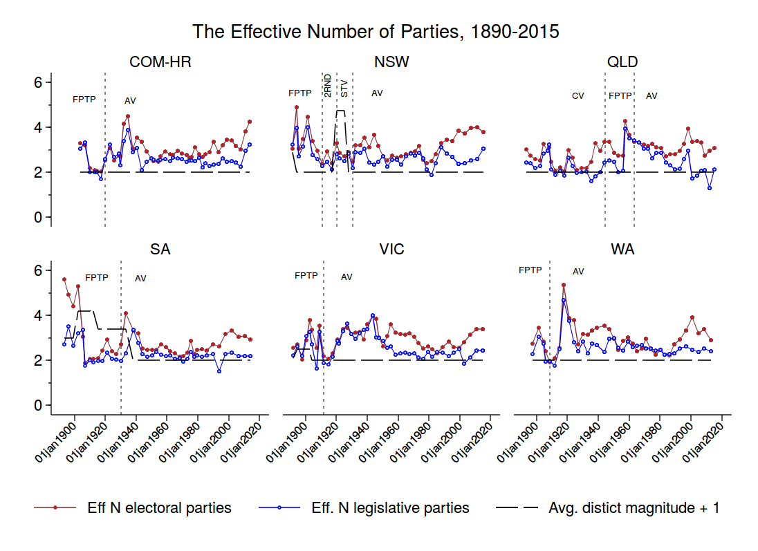
The Effective Number of Parties in Australia, 1890-2015
Figure 1 shows the effective number of electoral and legislative parties in the Australian Commonwealth and the five mainland states over time. These statistics provide a rough means to track the relationship between the electoral system and the party system. For example, we can use the data in Figure 1 to assess if changes to the electoral system precede sharp changes in in the number of parties that contest elections or win seats.
(Click on the figure to enlarge it)
From a theoretical perspective, one would not expect a shift from FPTP to AV to have a big impact on the effective number of parties. This is because both systems tend to be used in conjunction with single-member districts (i.e., districts magnitude = 1), and theory (Cox 1997) predicts M + 1 effective parties to contest elections. (And, because parties are unlikely to persist in contesting elections unless win at least some seats, to secure legislative representation, we might also predict M+1 legislative parties). The prediction is a weak one, however, because Cox’s M+1 rule operates at the district-level – and different sets of M + 1 parties could present themselves in different districts. Still, the dashed line in each panel of Figure 1 shows this M+1 threshold for each state.
Between 1940 and 1980, South Australia’s party system closely adhered to this theoretical prediction, with just 2.5 effective electoral parties and 2.25 effective legislative parties. However, the main message of Figure 1 is that the effective number of electoral and legislative parties can and does wander from this M+1 equilibrium. Observe, for example, the growth in the number of electoral parties in the post-1980 period at both state and federal levels. Plainly this post-1980 increase in electoral parties is not due to the main features of the electoral system because by this point in time all mainland state and federal elections in Australia were held under AV.
In addition, the effective number of electoral and legislative parties was pretty much the same under FPTP and AV controlling for differences in district magnitude. The effective number of electoral parties in each state and federally averaged about 3 (i.e., M + 2), and the effective number of legislative parties in averaged about 2.5 — and did so under both FPTP and AV.
Nor is there any evidence that changing the electoral formula from plurality to AV leads to changes in the effective number of electoral or legislative parties. Indeed, the evidence on this front is far more consistent with Cox’s view that it is mainly the district magnitude that shapes party competition. To show this, I ran regressions of year-to-year changes (i.e., first-differences) in the effective number of electoral (ΔENEP) and legislative parties (ΔENLP) on contemporaneous and lagged changes in the electoral formula (ΔF, ΔFt-1) and district magnitude (ΔM, ΔMt-1):
ΔENEPst = a + b1ΔFst + b2ΔFst-1 + b3ΔMst + b4ΔMst-1 + ust (1)
ΔENLPst = a + d1ΔFst + d2ΔFst-1 + d3ΔMst + d4ΔMst-1 + est (2)
The results (below) indicate that 1) an increase in the district magnitude in year t increases the number of electoral parties by .34 in t and the number of legislative parties by .21 in t+1.[4]
Table 2. OLS Model of Changes in the Effective Number of Electoral and Legislative parties
The Effective Number of Parties in Australia, 1890-2015
|
ΔENEPst |
ΔENLPst |
|
|
ΔFst |
–.29 (.15) |
–.14 (.17) |
|
ΔFst-1 |
.23 (.23) |
–.03 (.08) |
|
ΔMst |
.34*** (.07) |
.09 (.13) |
|
ΔMst-1 |
–.10 (.26) |
.21*** (.05) |
|
Constant |
–.005 (.01) |
–.01 (.006) |
|
N Obs |
239 |
239 |
|
R2 = .04 |
.04 |
.02 |
Robust SE clustered by state in parentheses
Conclusion
What these data suggest is that the introduction of AV in Canada is unlikely to generate major changes in the effective number of parties that contest elections or win seats. Canadian federal elections from 1949-2015 have been contested by 3.3 effective electoral parties, and produced an average of 2.5 electoral parties (not far off the Australian figures). The adoption of AV can be expected to leave these statistics intact precisely because such a reform would leave the district magnitude intact. This does not, of course, rule out changes in the identity of parties that contest elections or win seats or the possibility of major shifts in vote- or seat-shares between parties (because the effective number of parties remains the same whether the Liberals gain 35% of the vote, and the NDP, 15%, or the converse.)
In the next post, I’ll consider if/how the transition from FPTP to AV in Australia altered votes-seats proportionality.
[1] Under AV, voters (typically in single-member districts) rank their preferred candidates from 1-N. If any candidate secures 50+% of voters’ first-preferences, s/he is declared elected. If not, the lowest ranked candidate is eliminated and ballots cast for the eliminated candidate are distributed to the remaining candidates according to second-preferences. If any candidate secures 50+% of voters’ first- and second-preferences, s/he is declared elected. If not, the lowest ranked candidate is again eliminated and ballots redistributed, etc.
[2] Many thanks to my colleague, Campbell Sharman, for furnishing me all these data on Australian elections.
[3] The contingent vote (CV) is a hybrid between FPTP and AV: Under CV, the voter lists up to two preferences on their ballot, one for the most-preferred candidate and a second-preference for another candidate. If there is no majority-winner on first-preferences, then all candidates but the top-two are eliminated, and ballots cast for those candidates are redistributed according to second preferences. The winner is then the candidate with the plurality of first- and second-preferences.
[4] Using first-differences obviates the need to include state fixed-effects. Now, the model does restrict the coefficients to be the same across states, but there’s not really enough variation to allow for the coefficients to vary by state. Also, it’s clear that changes in formula include shifts from say, STV to CV, as in NSW; they are not just confined to transitions from FPTP to AV. But the results are largely unaffected by, say, dropping NSW from the model.
 Follow