
Apart from the Points of Interest, important factors that also need to be considered are: land use, population in residential areas and number of renters.
To use in our Multi Criteria Evaluation, these three factors must be normalized and then converted into raster format.
Land Use
The 2011 Land Use data collected included 24 land use types. For our analysis, this large number was not needed. We decided to group together similar land use types. Six different classes were created for symbology purposes. The weight importance of each class compared to each other was determined using the Analytic Hierarchy Process (AHP) on 123AHP. A list of the grouped land use types, as well as their corresponding weights, are as follows:
- Mixed Residential Commercial (0.4865)
Includes Mixed Commercial and Residential low rise and high rise apartments. - High Density Residential (0.2334)
Includes Residential High-Rise apartments, Low-Rise apartments, Townhouses. - Commercial (0.1389)
Includes Institutional, Commercial. - Low Density Residential (0.0820)
Includes all other residential types such as Mobile Home Park, Single Detached and Duplex, Rural, Institutional and Non-Market housing. - Industrial (0.0416)
Includes Airport/Airship, Industrial, Industrial Extractive and Rail, Rapid Transit, Other Transportation, Utility and Communication. - Prohibited Construction and Development (0.0175)
Includes all other land use types which cannot be constructed on such as Agriculture, Cemetery, Harvesting and Research, Lakes and Other Water, Port Metro Vancouver, Protected Watersheds, Recreation, Open Space and Protected Natural Areas, Road Right-of-way, Undeveloped and Unclassified.
This resulting edited Land Use layer was converted into a raster layer using Polygon to Raster within Conversion Tools (Figure 8). The Value Field used was the corresponding weights from the AHP. The Cell Assignment used was Maximum Combined Area with a cell size of 10m.
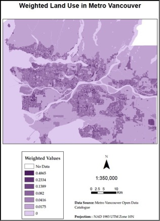
Figure 8. Results from Polygon to Raster for Land Use. Higher weight is given towards mixed residential commercial areas, symbolized in dark purple.
Population Density in Residential Areas
The population dwelling counts in each DA were downloaded as a table (from CHASS) and joined to the DA shapefiles (from Geography G drive) by the attribute “DAUID”. Using the polygon Land Use layer, a residential-only land use layer was extracted by selecting the residential attributes. Using Intersect, the residential-only land use layer is joined with the DA population shapefile. This will give a count of how many residential areas are located within each DA. Using the Summarize function, the number and area of residential areas within a DA are summed. The population density within residential areas can be found by dividing the number of persons by the total area of residential units within the DA, to give a density (in persons/sq m). To address the outliers in our data, population density values were changed to 0 for the following DAUID:
- 59150014
- 59151710
- 59153569
- 59153592
- 59153608
- 59153616
- 59153633
The population density layer is then converted to raster, with the same parameters as the Land Use layer (Figure 9).
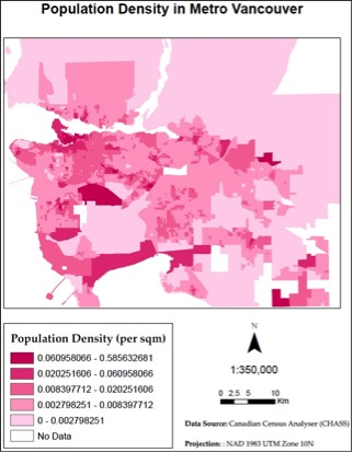
Figure 9. Results from polygon to raster for Population Density in residential areas. Numbers represent the amount of people dwelling in residential areas per square metre.
Renter Percentage
The data for the number of renters per CT were downloaded as a table from CHASS. After joining with the CT shapefiles, the population counts per CT was joined with the Renter attribute table using the Value Field “CTUID”. The number of renters was then divided by the population to give a renter density. Like the Population Density layer, outliers were addressed by changing the renter density value to 0 for the following CTUID:
- 9330150.00
- 9330161.01
- 9330250.02
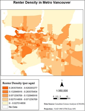
Figure 10. Results from polygon to raster for number of renters per CT.
The resulting renter layer is then converted to raster, with the same parameters as the Land Use and Population Density layers (Figure 10).