Data Acquisition
Listed below is a table of our current obtained datasets to conduct this project (refer to table 1). Our list of datasets are acquired from a variety of credible sources including CHASS Canadian Census Data Center, Vancouver Open Data Portal, Metro Vancouver Open Data Catalog and Statistics Canada. They are acquired based on our need to conduct and demonstrate our analyses taking into account our area of study (Vancouver), infrastructures within our area of study, explanatory variables (income, population density, level of education attainment and visible minority population) and our dependent variable (Greenest City Projects).
Consequently, we are aware that the census data we are obtaining is quite outdated as it is obtained from the year 2016 for all of our variables. We are taking this into consideration as a limitation and a recommendation to future studies in this field.
| Layer/Datafile Name | Description | Attributes (that will be utilized) | Data Source | File Type, Entity | Year of Publication |
| Visible Minority (CT) | 2016 Statistics Canada Census Data of the total population of visible minorities by Census Tract | COL2 – Visible Minority | CHASS | .csv, Raster | 2016 |
| Population Density (CT) | 2016 Statistics Canada Census Data of the total population density by Census Tract | COL1 – Population Density per square kilometer | CHASS | .csv, Raster | 2016 |
| Population (CT) | 2016 Statistics Canada Census Data of the total population density by Census Tract | COL1 – Total Population | CHASS | .csv, Raster | 2016 |
| Education Levels (CT) | 2016 Statistics Canada Census Data of the highest educational attainment by Census Tract | COL1 – Highest Educational Attainment for population ages 25 to 64 | CHASS | .csv, Raster | 2016 |
| Levels of Income (CT) | 2016 Statistics Canada Census Data of the total income of households by Census Tract | COL1 – Total income statistics for the population aged 15 years and over in private households | CHASS | .csv, Raster | 2016 |
| Greenest City Projects | Point data on the location of every “Green City” project implementation between 2011 and 2020 | Entire Dataset Used | Vancouver Open Data Portal | .shp, Vector points | 2021 |
| 2016 Generalized Land Use Classification | Polygon file of all land use classifications within the Metro Vancouver Region | Entire Dataset Used | MetroVancouver Open Data Catalogue | .shp, Vector Polygons | 2016 |
| Vancouver Area Boundary | Polygon shapefile of all Canada province boundaries | Polygons within the Metro Vancouver Region | Statistics Canada | .shp, Vector polygons | 2011 |
| Coastal Waters | Boundary File of Canada’s coastal waters | Entire Dataset Used | Statistics Canada | .shp, Vector Polygons | 2011 |
| Public Streets | Vector file displaying all major roads and streets within Vancouver | Entire Dataset Used | Vancouver Open Data Portal | .shp, Vector Line | 2019 |
Table 1: List of Datasets used within our final project which will be mapped onto ArcGIS Pro
Normalizing Population Density Data
To begin the analysis of our variables, we required an accurate population density of each Census Tract that could be adequately compared against “Greenest City” project locations. This was done as a countermeasure of Statistics Canada’s methods of calculating population density, which is done by dividing the population of a neighborhood boundary (CT or DA) by the square footage of that area. This poses an issue with accuracy when considering the variety of land uses within an area, given that this method assumes all land use to be residential (EPA Gov, 2015). To counter this issue, we conducted dasymetric mapping to the Statistics Canada Population data that would consider only residential land coverage in population density calculations (Process shown in Chart 1). Displayed below (Map 3) is a display of residential vs. non-residential land use distributions highlighting its discrepancies, and how this can drastically skew population density data and our intended analyses. As visualized by Stanley Park (shown in inset Map 3), we can see how its low population density rate does not reflect the entire region, rather it is the vast non-residential parkland that skews the high density that exists in one corner of the CT and alters how the boundary area is considered in our calculations.
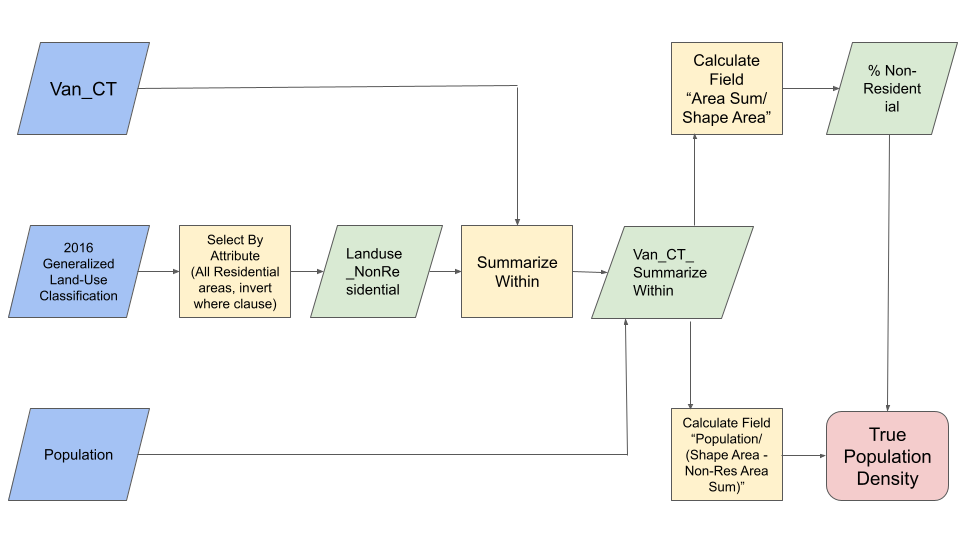 Chart 1: Flowchart depicting the steps taken in normalizing population density to accurately reflect land-use
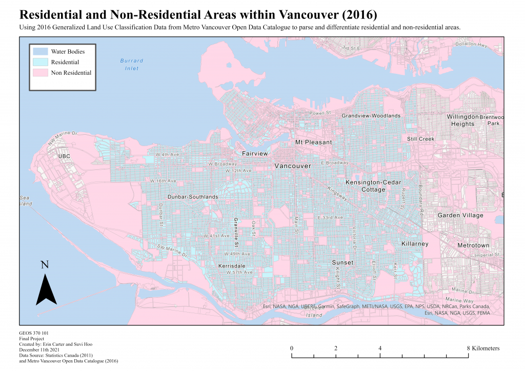 Map 2: Map Depicting the Distribution of Residential and Non-Residential Land-use areas to be utilized in our Population Density Normalization
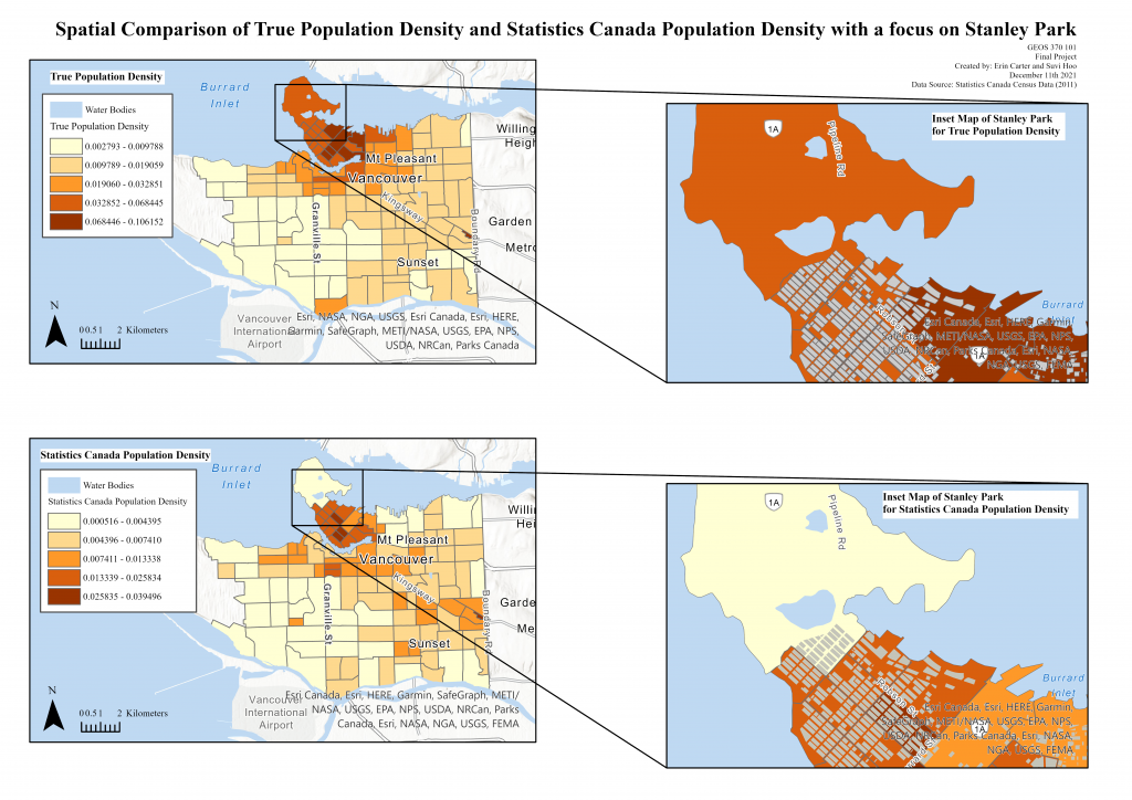
Map 3: Map depicting the spatial difference in Statistics Canada Population Density and our Normalized True Population Density. Map Units are displayed in Percentages.
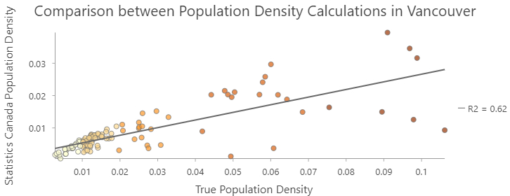
Chart 2: Scatterplot depicting the difference between the values of Statistics Canada Population Density and our Normalized True Population Density
Spatial Comparison of Explanatory Variables
Prior to utilizing statistical analyses, we found it helpful to create visual comparisons of our four variables against “Greenest City” project areas in order to make inferences as to whether notable spatial divisions exist. Each variable was presented on our base map and given graduated colors on a 5 class value scale. Results showed that for each variable, values appear to be clustered which indicates to us the likely occurrence of spatial autocorrelation. Specifically, it appears as though the higher values of each predictor are found near areas in which Greenest City projects are the most frequent (Map 4).
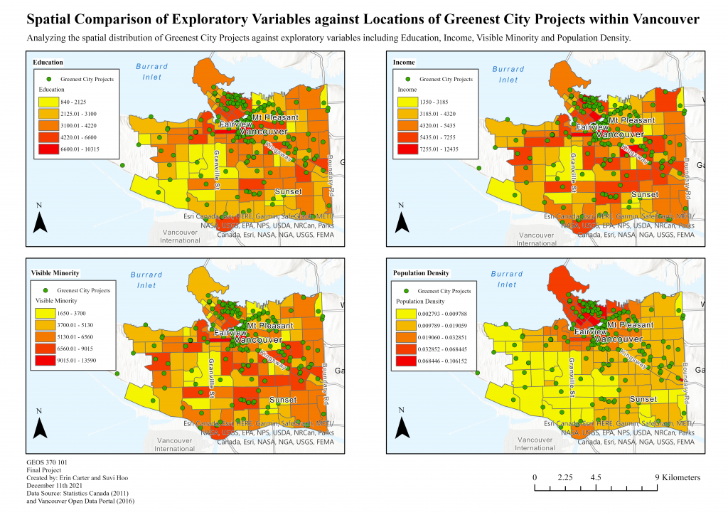 Map 4: Spatial Comparison of Exploratory Variables Against Greenest City Project Locations. Map Units for Education, Income, Visible Minority are full population numbers, Map Units for Population Density is in Percentages.
Spatial Autocorrelation
Commencing our spatial analysis, we began by utilizing the Spatial Autocorrelation tool in order to determine whether our variables are influenced by systemic spatial variation, and visualize potential clusterings of values.
Exploratory Regression Analysis
In order to evaluate the significance of our explanatory variables and compare for any evidence of multicollinearity, we chose to utilize an exploratory regression analysis. An exploratory regression analysis is a data mining tool that tests all combinations of explanatory variables to determine which models pass outlines necessary OLS Diagnostics, and indicate consistent predictor variables as well as whether any explanations are missing. The parameters for our analysis are as follows:
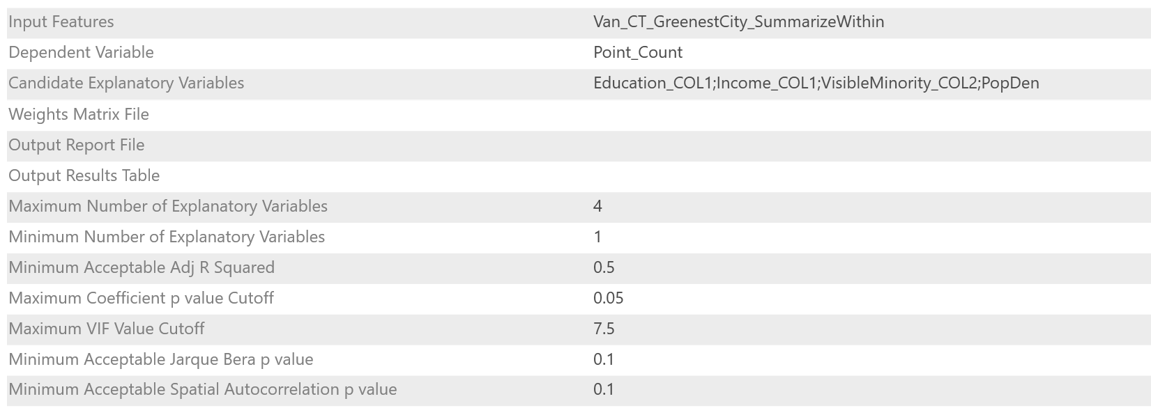 Parameter 1: Imputed parameters in conducting an Exploratory Regression Analysis for Greenest City Projects against Explanatory Variables.
Generalized Weighted Regression Analysis
Following our Exploratory Regression Analysis, we performed a Generalized Weighted Regression Analysis which would allow us to examine the ways in which the relationships between our dependent variable and predictor variables might vary over space. This analysis would additionally allow us to take a step further in drawing conclusions around whether the variable coefficients change depending on their spatial location. The parameters for our analysis are as follows:
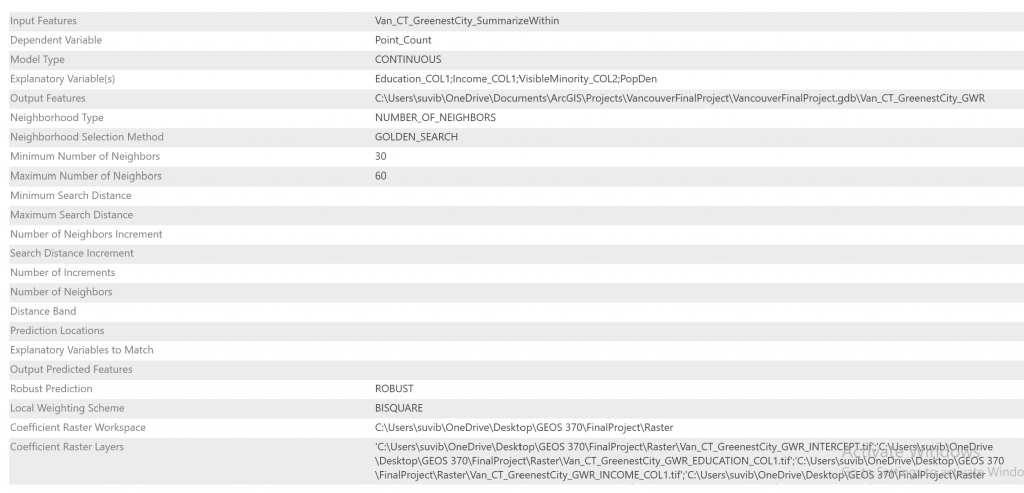 Parameter 2: Imputed parameters in conducting a Generalized Weighted Analysis for Greenest City Projects against Explanatory Variables.