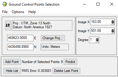
The process of Image Georectification or Georegistration involves associating a remotely sensed image with a particular coordinate/reference system.

The final Ground Control Points (GCP) Selection Window:

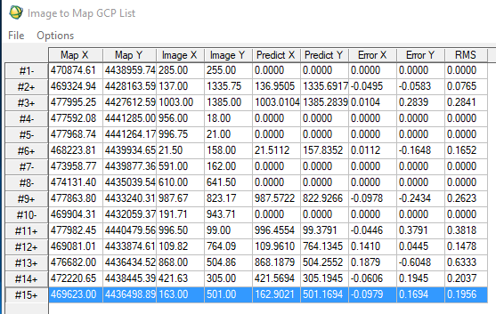
The GCP List (Showing all Root Mean Squared (RMS) Errors and the Total RMS):

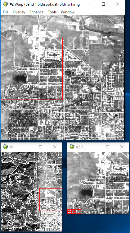
The Final Resampled Image with Overlaid Roads Demonstrating Closeness of Fit:

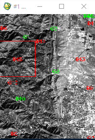
The Roads Layer Showing GCP Distribution:

*Data based on Panchromatic SPOT (Système Pour l’Observation de la Terre) imagery of Boulder, Colorado, U.S.A (UTM Zone 13 North), with a spatial resolution of 10 meters. Image Georectification carried out using ENVI Classic.

Section 1: Image Classification

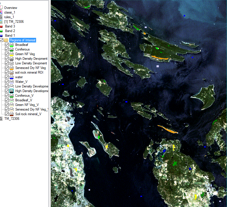
Classification of the Landsat TM image using the Maximum Likelihood classification algorithm and the following 6 bands as inputs: Blue, Green, Red, NIR, SWIR1 & SWIR2 [Landsat Band 7]:

Classification Polygon Graph:

Class	# Required Polygons	# Required Pixels	Total Polygons Used	Total Pixels Used
Water	10	>500	10	1087
Broadleaf Forest	10	>500	10	781
Coniferous Forest	10	>500	10	815
Green non-Forest Vegetat.	5	>250	5	679
Senesced-Dry Non-Forest Veg	5	>250	5	879
High Density Development	5	>100	5	1035
Low Density Development	5	>100	5	999
Soil Rock Mineral	5	>100	5	691
Water_Validation	5	>250	5	548
Broadleaf_V	5	>250	5	432
Coniferous_V	5	>250	5	948
Green NF Veg_V	2 or 3	>125	2	233
Senesced Dry NF Veg_V	2 or 3	>125	3	140
High Density Devpment_V	2 or 3	>50	3	540
Low Density Devpment_V	2 or 3	>50	3	766
Soil Rock Mineral_V	2 or 3	>50	3	103

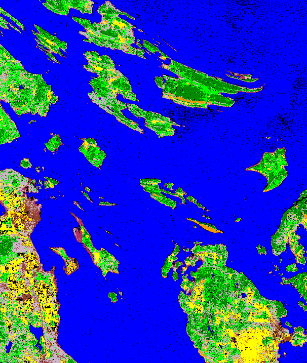
Final Classified Image:

Section 2: Classification Accuracy Assessment

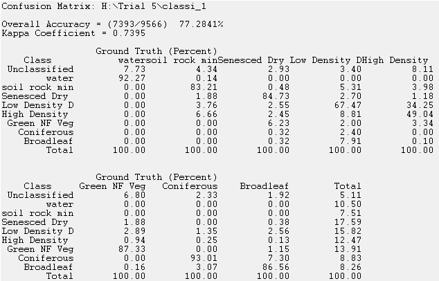
*Findings based on Landsat TM raster data representing the southern Gulf Islands, BC, Canada acquired in July, 2006.

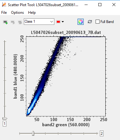
Section 1: Exploring Feature Space Scatter Plots
Blue vs. Green Bands:

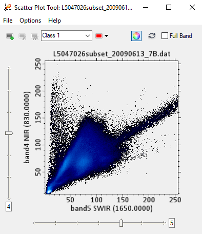
Near InfraRed vs. Short-Wave InfraRed:

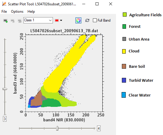
Section 2: Labeling the Feature Space Scatter Plot of the Red vs. Near InfraRed Bands by Land Cover Classes

*Scatter Plots based on Panchromatic Landsat 7 raster data of Vancouver, BC, Canada.

Section 1: The Electromagnetic Spectrum (EMS)

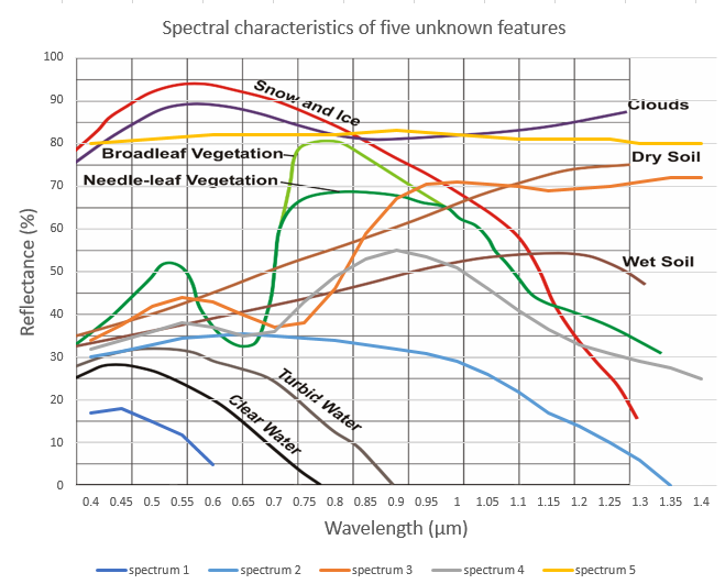
Broadleaf Vegetation is reflected the most at wavelength of 0.8 - 0.85 µm, belonging to the Near-InfraRed region of the Electromagnetic Spectrum. Needle-leaf Vegetation is reflected the most at wavelength of 0.85-0.95 µm, belonging to the Near-InfraRed region of the Electromagnetic Spectrum.

Dry soil and Vegetation have different reflectance characteristics at ranges 0.5-0.6 µm, 0.65-0.75 µm, 0.8-1.0 µm, and 1.1-1.4(+) µm, which belongs to the Visible Light, Visible Light to Near-InfraRed, Near-InfraRed, and Near-InfraRed portions of the Electromagnetic Spectrum respectively.

Broadleaf and Needle-leaf vegetation both reflect the same amount of Energy at 0.6 µm because they both share the same (general) colour of green due to the shared chlorophyll content of the Vegetation. They fall in the Visible Light section of the Electromagnetic Spectrum.

At 0.85 µm, Clouds, Snow and Ice look almost identical, while Dry and Wet Soil look almost identical. At 0.4 µm, Clean and Turbid water look almost identical with each other, Needle-leaf Vegetation, Broadleaf Vegetation, Dry and Wet soil look almost identical with each other, and Snow and Ice look almost identical with each other.

Hypotheses:
Spectrum 1: I hypothesize that Spectrum 1 represents clean water.

Spectrum 2: I hypothesize that Spectrum 2 represents very turbid muddy water or some form of impure melting snow.

Spectrum 3: I hypothesize that Spectrum 3 represents a lighter green variety of Lawn Grass according to the Landsat Spectral Characteristics Viewer.

Spectrum 4: I hypothesize that Spectrum 4 represents a lighter green variety of Fir Spruce according to the "Fir Spruce" curve found in the Landsat Spectral Characteristics Viewer.

Spectrum 5: I hypothesize that Spectrum 5 represents impure Calcite as it has a slightly lower curve compared to the ‘Calcite’ curve found in the Landsat Spectral Characteristics Viewer.

Section 2: Landsat 7 Bands, the EMS & ENVI Software

I believe that the best composite for mapping vegetation is when Red is assigned to represent Band 4 NIR (760-900 nm), Green is assigned to represent Band 2 Green (520-600 nm), and Blue is assigned to represent Band 6 TIR (1040-1250 nm). I allocated Green to Green as doing so allowed me to assess vegetation vigour and chlorophyll content. Moreover, it is quite a natural colour to apply to visibly green surfaces. I allocated Red to Near-InfraRed as the chlorophyll content in vegetation is highly reflective and makes vegetation easily distinguishable from bodies of water. Lastly, I allocated Blue to Thermal as doing so allowed me to assess vegetation status and disturbance magnitude in forest fire-prone zones. Such a reading may not be very useful in Vancouver as forest fires are not common, but Thermal InfraRed (TIR) is useful to observe in Canadian Boreal forests as well as in the Interior Northwestern region of the US. All three choices were also chosen because they are relatively secluded on the spectral signature graph at those wavelengths. All in all, chlorophyll-rich vegetation is observed as cranberry red, chlorophyll-less vegetation is observed as lime green, urban areas are observed as dark purple, water is observed as black, and snow and clouds are observed as yellow.

Section 3: Exploring More False Colour Composites

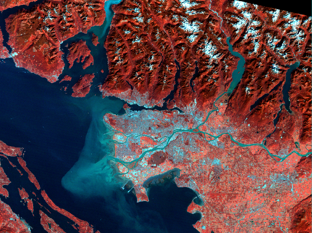
a. For analyzing Water Quality, I used band combination:
Red = 760-900 nm
Green = 520-600 nm
Blue = 450-520 nm

This band combination was chosen because – aside from Green and Blue representing their visible colours and Red as a common colour associated with NIR wavelengths among the remote sensing community – water quality can be assessed given the brightness of the blue/green in the water representing higher levels of water turbidity. Moreover, when mixed with substantial chlorophyll content, the pixels are observed to look rusty-orange in colour (as is the case of South Delta).

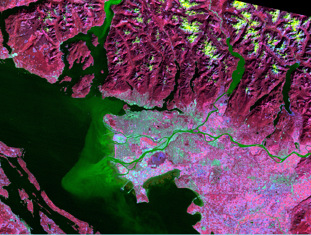
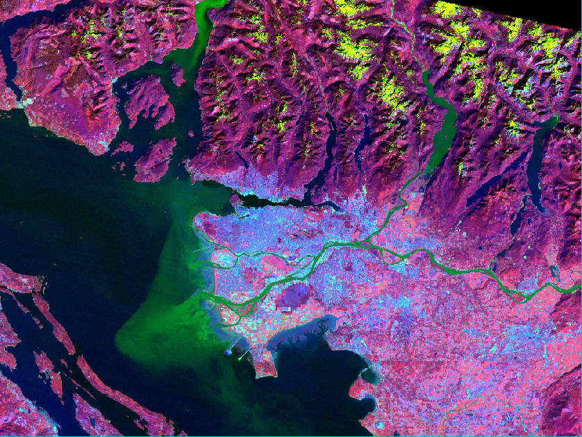
b. For analyzing Agriculture, I used the band combination:
Red = 760-900 nm
Green = 520-600 nm
Blue = 1550-1750 nm

This resulted in the easily identifiable hot pink pixels representing agricultural land while the blood red pixels represented forest land, and all other green areas represented urban areas (indigo), turbid water (cyan), or snow/clouds (light).

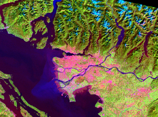
c. For analyzing Urban Areas, I used Red for Thermal-InfraRed to see the Urban Heat Island (UHI) effect of urban areas, and juxtaposed it with Green for Chlorophyll-reflective NIR to compare it to vegetation zones, as well as Blue for Blue to contrast the urban and vegetation zones with water and snow zones.

*False Colour Composites are of the Greater Vancouver Area, BC Canada.