Theory
For our rainfall analysis I used the modelling techniques developed by Montgomery and Dietrich (1994) in A physical based model for the topographic control on shallow landsliding. This model classifies the slope based on the governing equations in Table 3 below.
Table 3: Governing equations for slope stability
| Condition | Equation |
|---|---|
| Unconditionally Stable | tanα ⩽ tanα [1-γw/γr] [9] |
| Unconditionally Unstable | tanα > tanφ [10] |
| Unstable if | a/b ⩾ T/q sinα (γw/γr) [ 1 – tanα/tanφ] [11] |
- α is the slope angle,
- γw is the unit weight of water,
- γr is the unit weight of the surface material,
- φ is the friction angle of the surface material,
- a is the flow accumulation
- b is the width of the cell through which flow passes
- T is transmissivity (m2/d)
- q is the critical steady-state rainfall (mm/d)
In order to use this model a few special adjustments to our dataset must be made. We first assume that that the soil is fully saturated so there is zero cohesion, which we remove from the fundamental equations to get the simplified equations above. However, rocks will still have cohesive strength, so we adjust for that by increasing the friction angle of rock to 80º. Additionally, roots will provide cohesion, so we adjust for this by adding an additional 5º to the friction angles of the parent materials, giving us the modified friction angle.
Hydrological Model
Before running the analysis I needed to find the flow accumulation for each cell. This involved preparing a hydrological model. To do this I first filled the sinks in the DEM using Hydrology toolset Fill tool, which is used to ensure the proper delineation of basins and streams. I then used the Flow Direction tool to find the flow direction of each cell, which was required to run Flow Accumulation tool.
Flow Accumulation outputs a grid that contains the accumulated number of cells upstream of a cell for each cell in the input grid. To convert this into the raster layer a/b I used the Raster Calculator to multiply the Flow Accumulation by the area of each cell (10m x 10m), then divided it by the width of one cell (10m).
Slope Stability Model
I then created the model in Figure 5 to find the Stability Index (SI) based off differing rainfall levels.
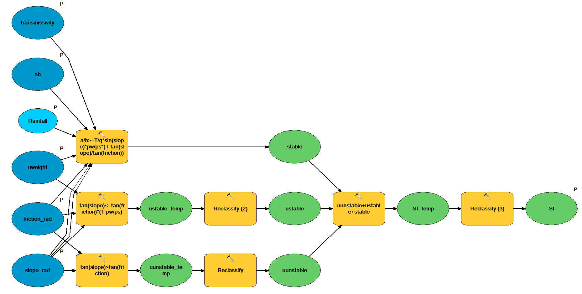
Figure 5: Stability Index Model
This model uses the slope angle angle, the modified friction angle, unit weight, and transmissivity of the parent material, the a/b layer, and the daily rainfall as inputs. It then uses the Raster Calculator to run the given equations in Table 3, and outputs a 0 if false and 1 if true. In order to keep track of the different conditions, it reclassifies the outputs by assigning them different values. After the three equations are computed, it adds the output rasters. Based off the output values it then determines whether a slope is unconditionally stable, unconditionally unstable, stable, or unstable based off the daily rainfall.
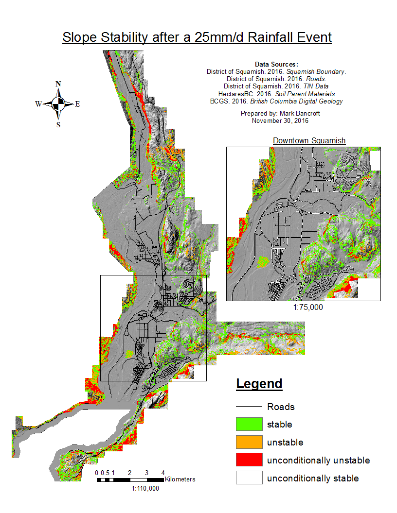
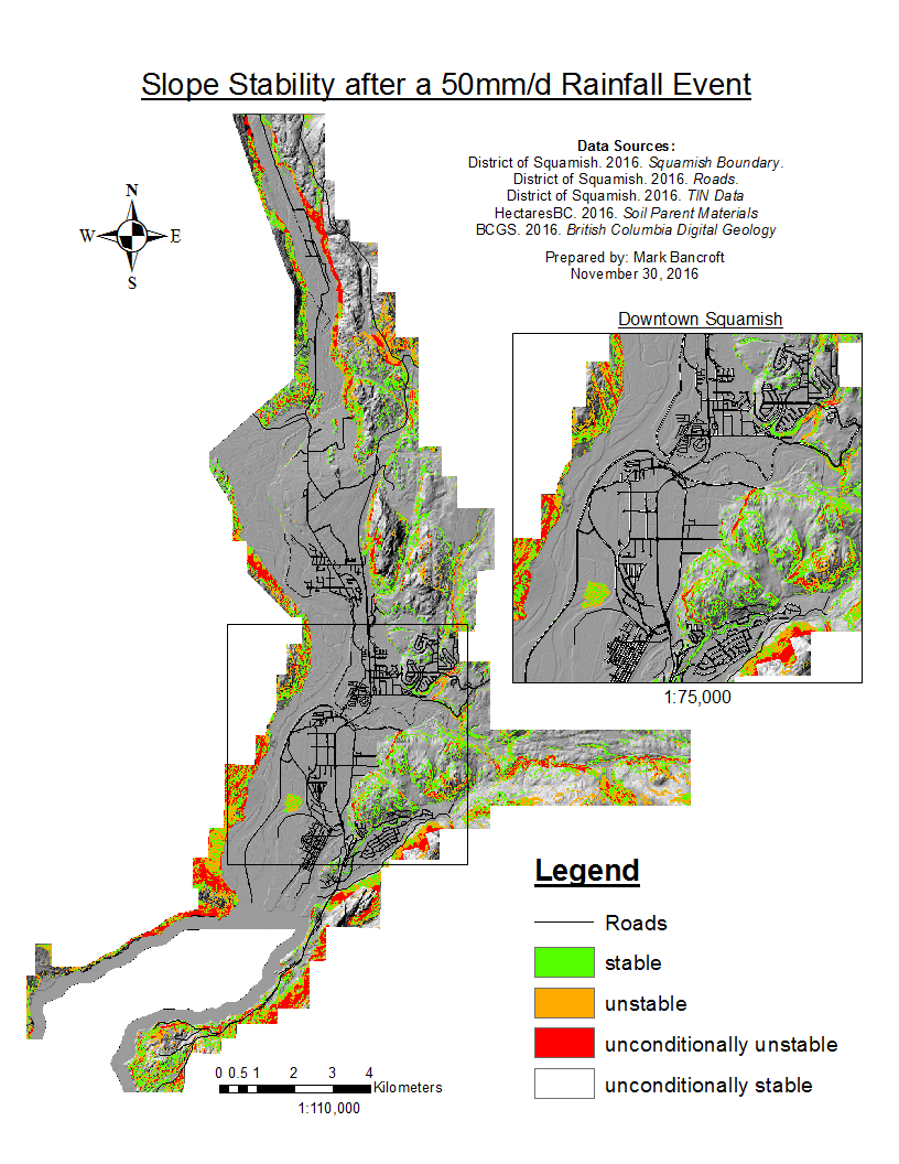
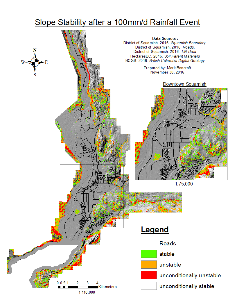
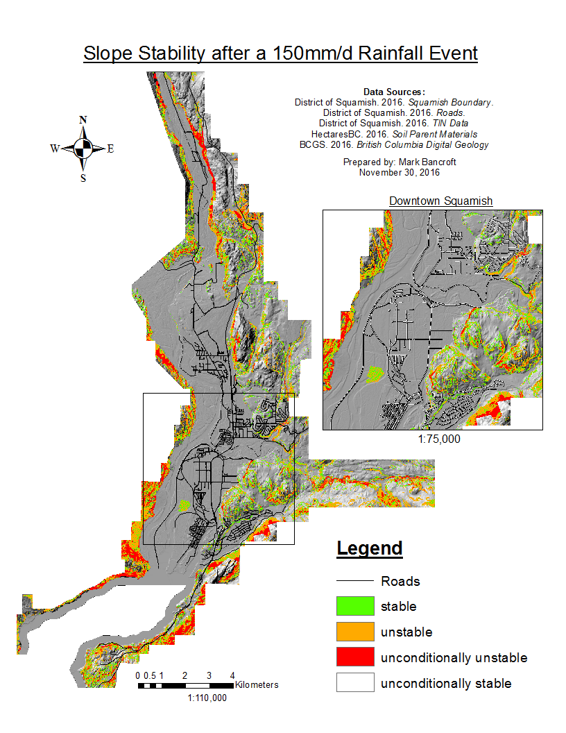
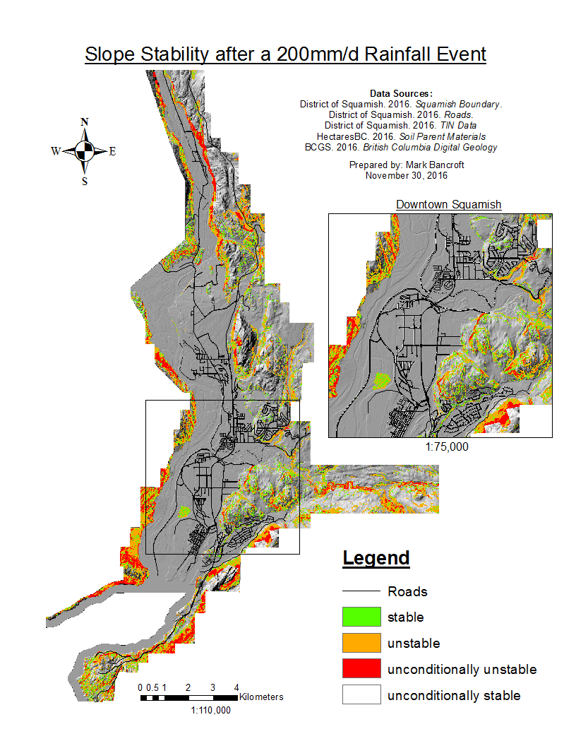
Results
The results for the differing rainfall levels are displayed in the accordion below. The 25mm/d rainfall represents a standard rainfall, while the 200mm/d rainfall represents a 1:25 year return period (Environment Canada). The majority of the land is unconditionally stable, with only the steep cliffs classified as unconditionally unstable. As the rainfall increases to 200mm/d, a larger area of the cliffs, especially on the eastern and western slopes, become unstable.