The 2D “Roughness Spectrum”
I) Preamble
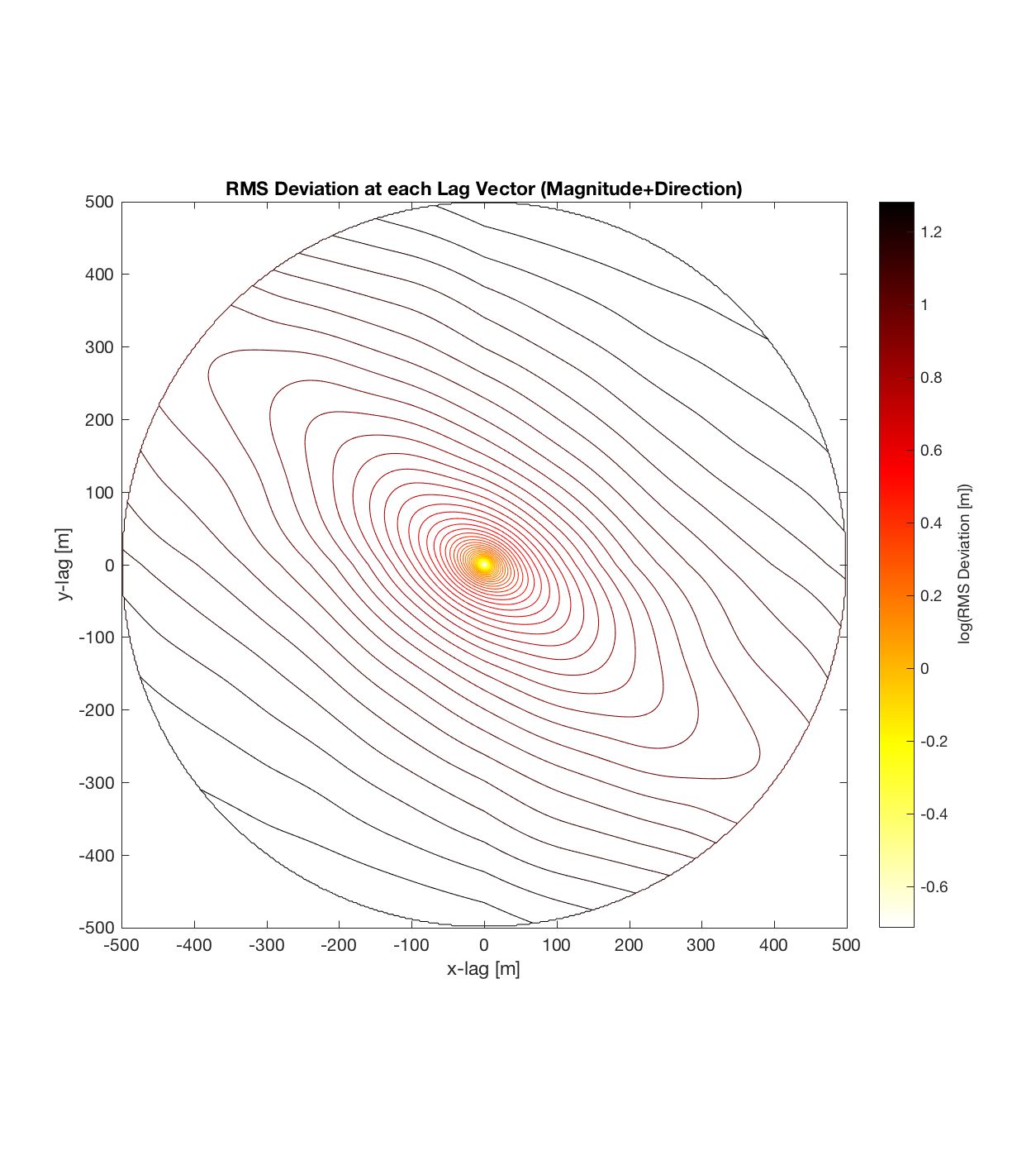
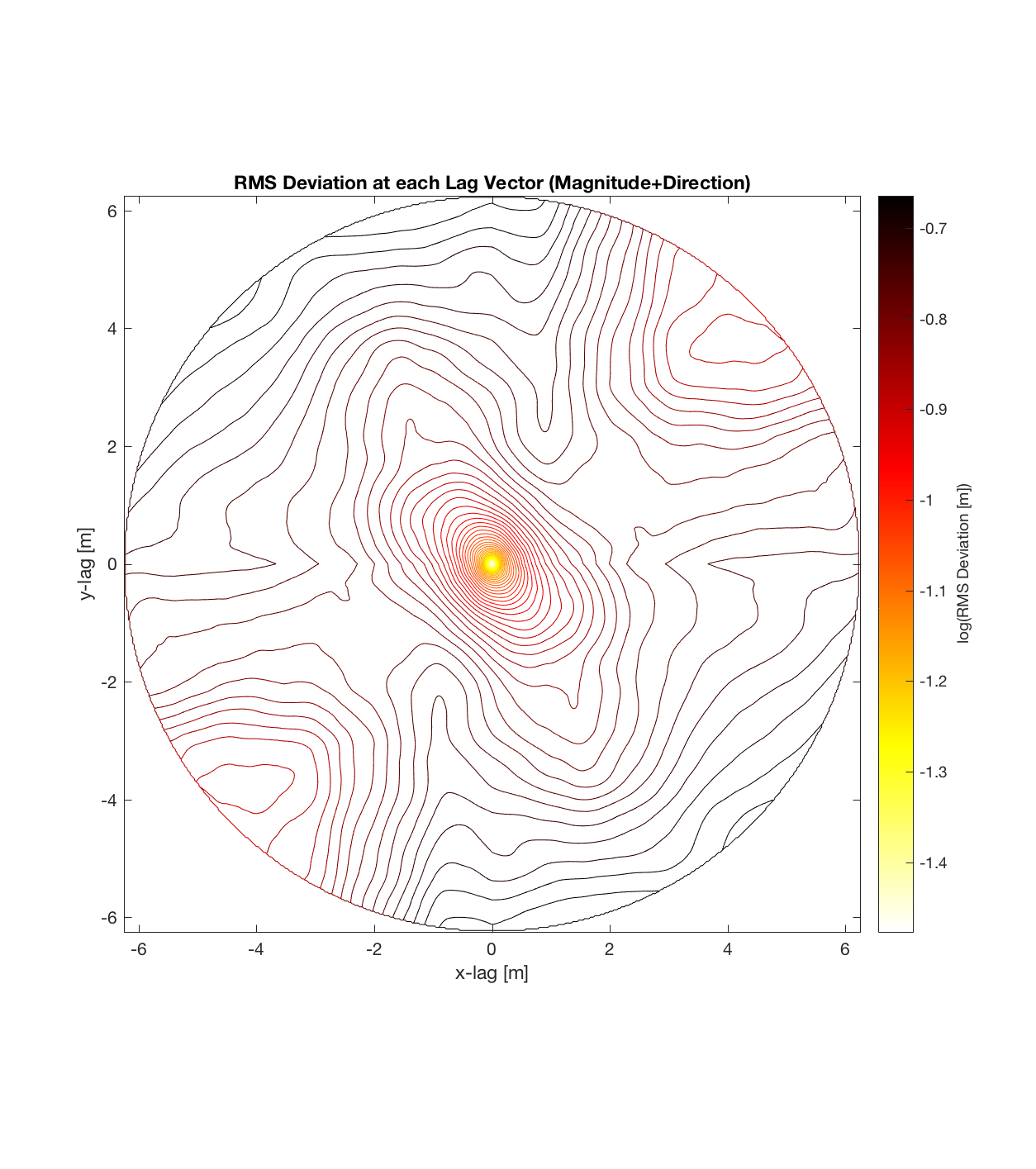
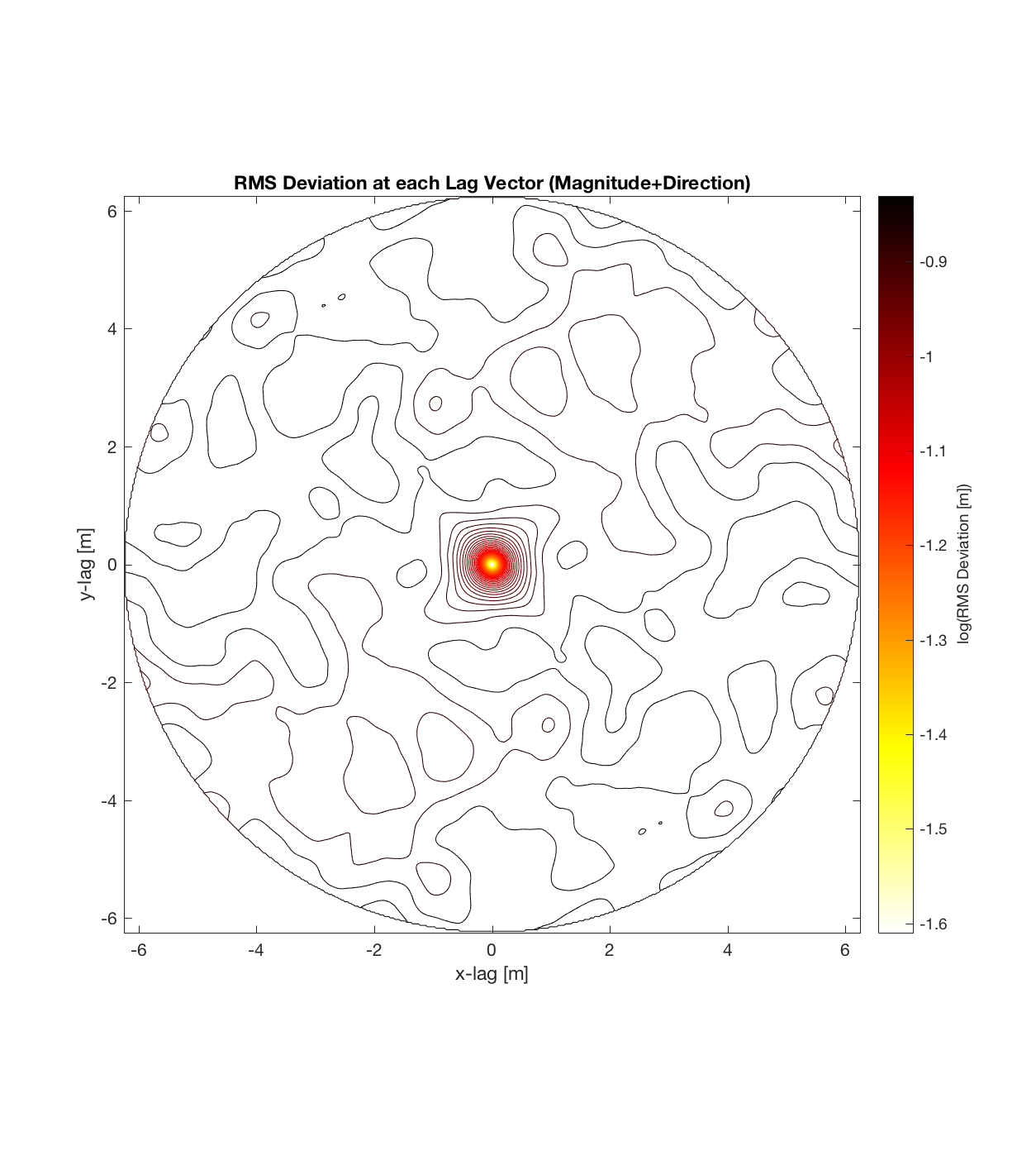
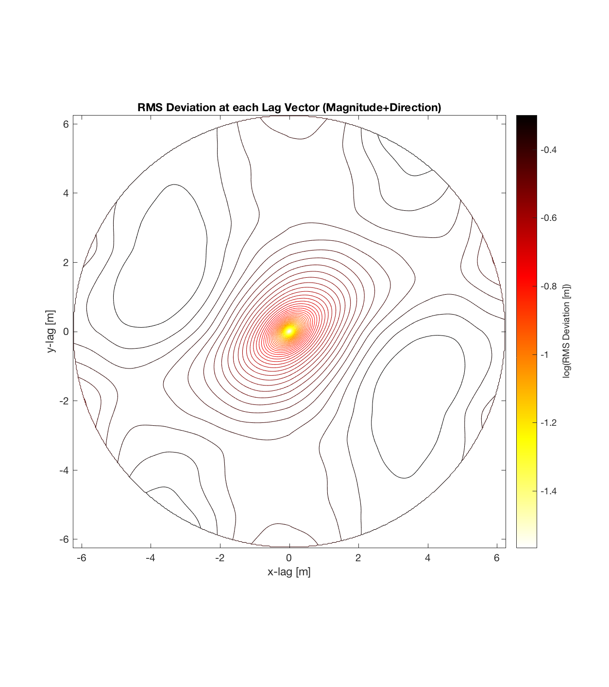
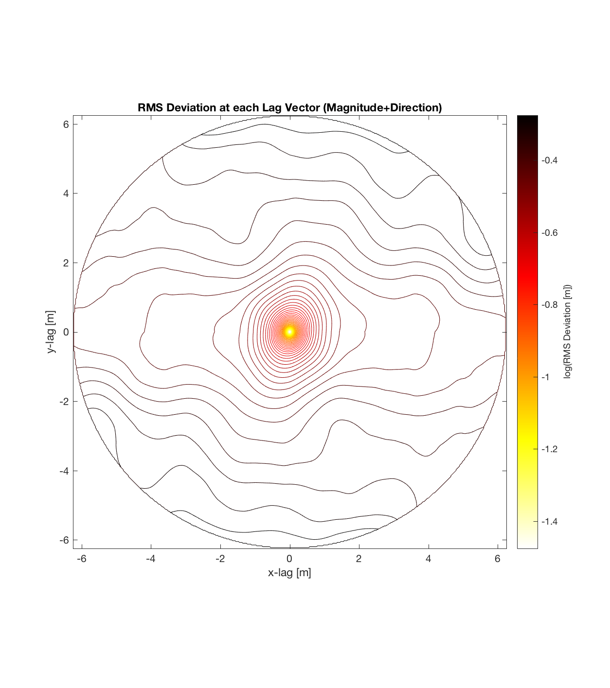
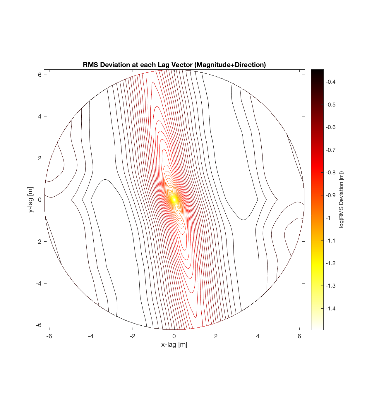
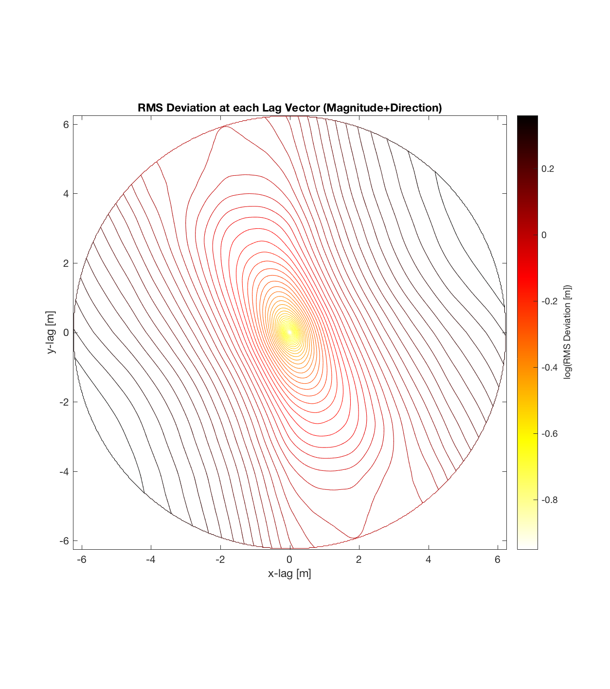
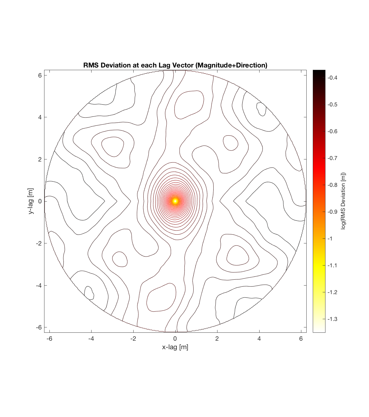
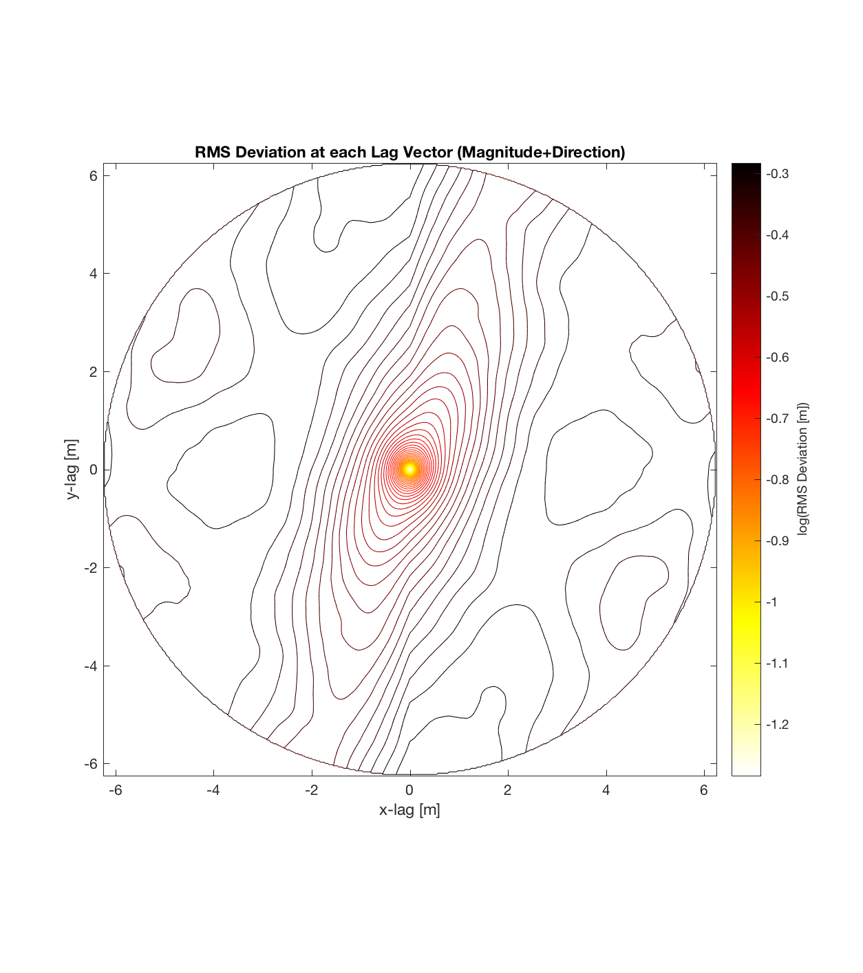
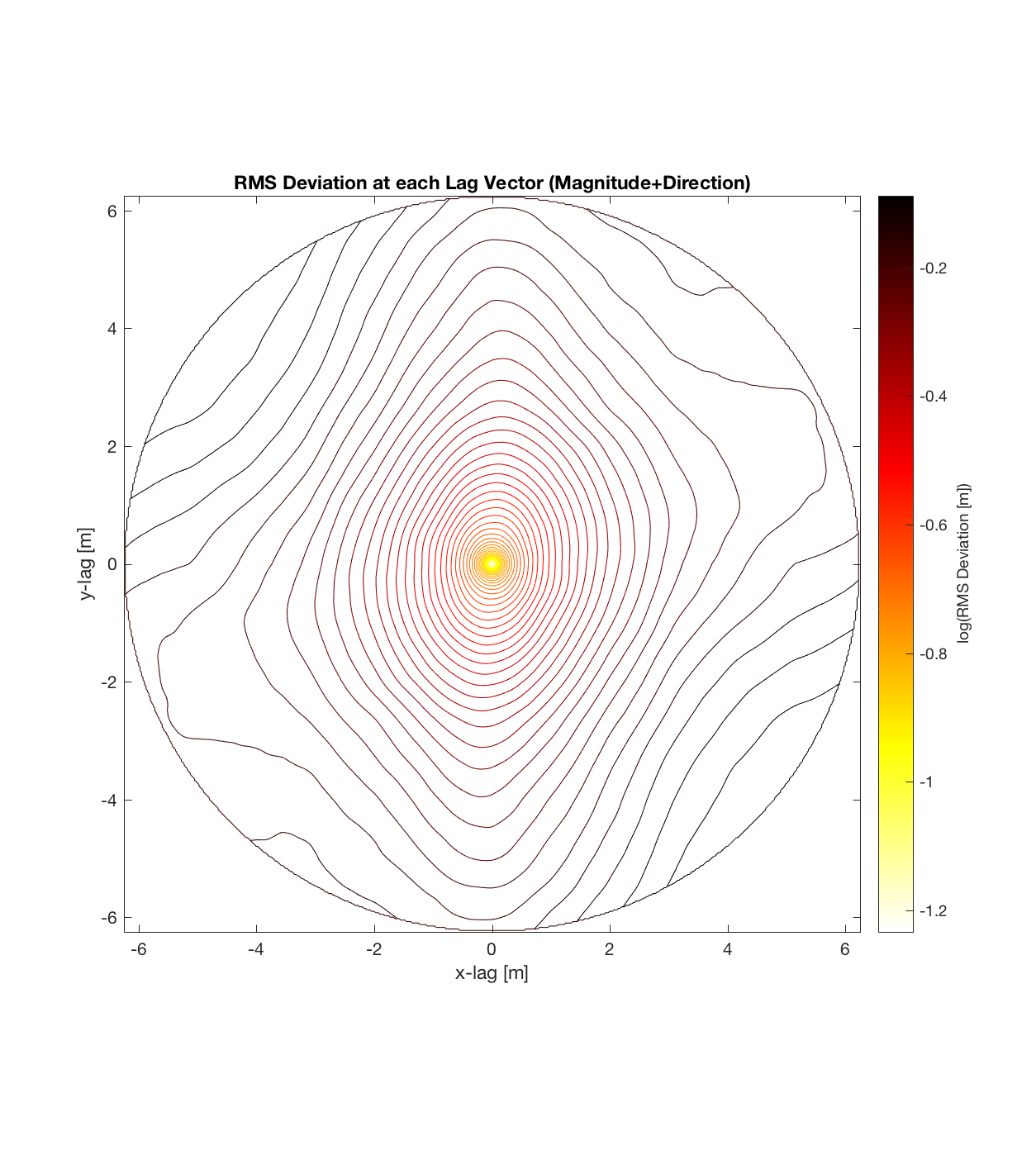
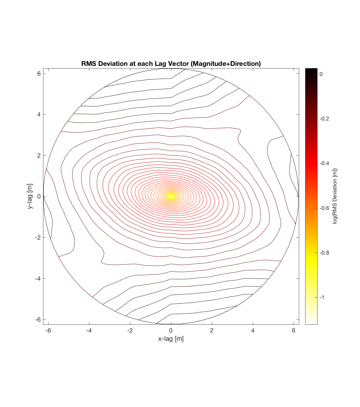
I came across a very insightful paper pertaining to 2D surface roughness characterization. Entitled “Characterization of the Structure of River-Bed Gravels Using Two-Dimensional Fractal Analysis” (Butler, Lane, and Chandler 2001), it one way to illustrate 2D roughness and associated anisotropy in such: contour diagrams (logarithmically-spaced), over a specified lag space.
Since the method is essentially the same as that which I (mistakenly thought I) came up with, the only steps required are plotting the RMS Deviation (which is the square root of the semivariance employed by Butler) as a function of lag vector magnitude (rather than of space), and employing the maximum sampling density in the algorithm. While this plot is not as intuitive to interpret, due to the fact that the ‘x’ and ‘y’ axes are not spatial variables, The method has some key advantages:
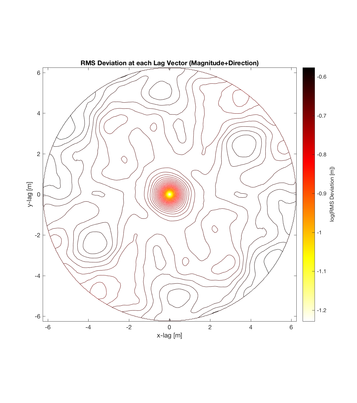
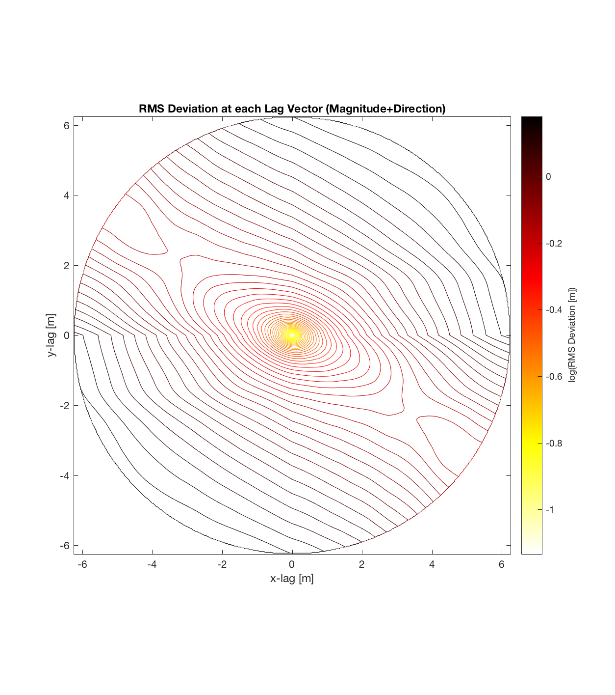
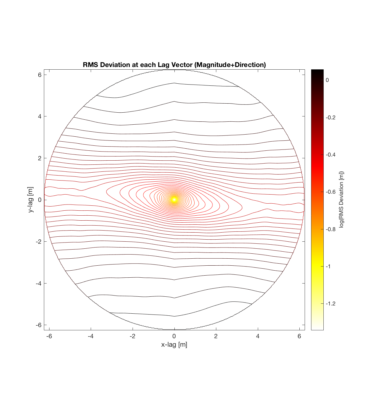
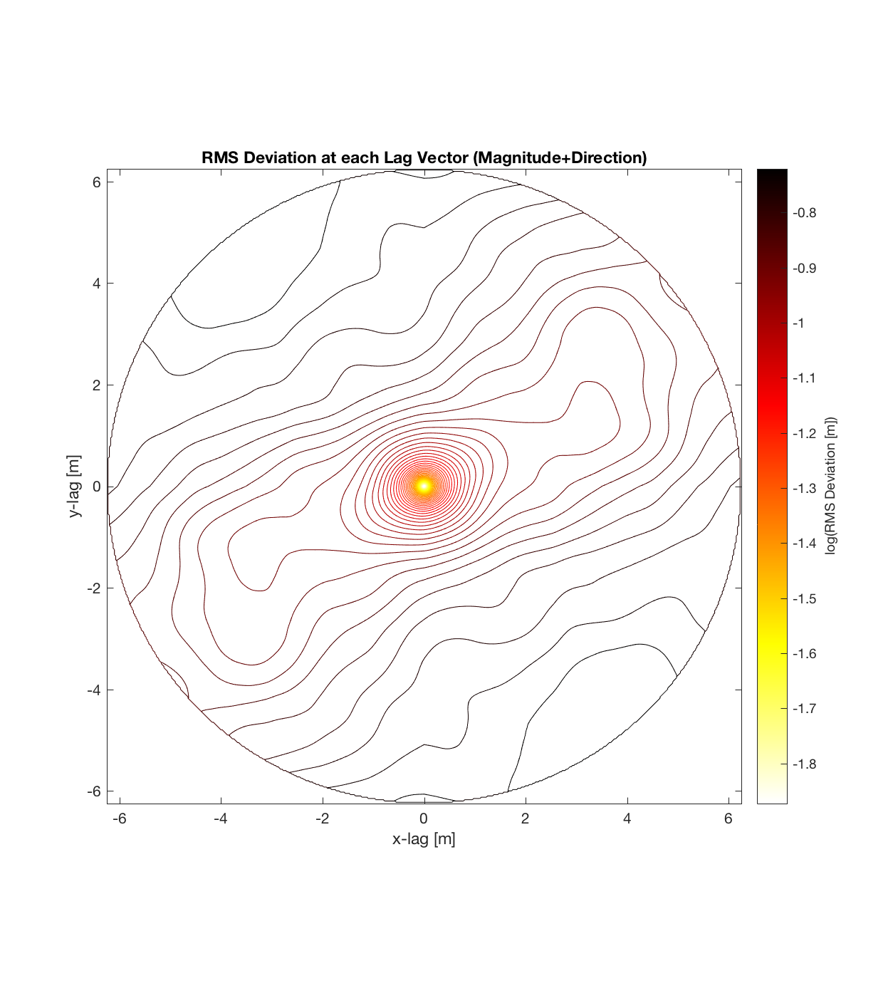
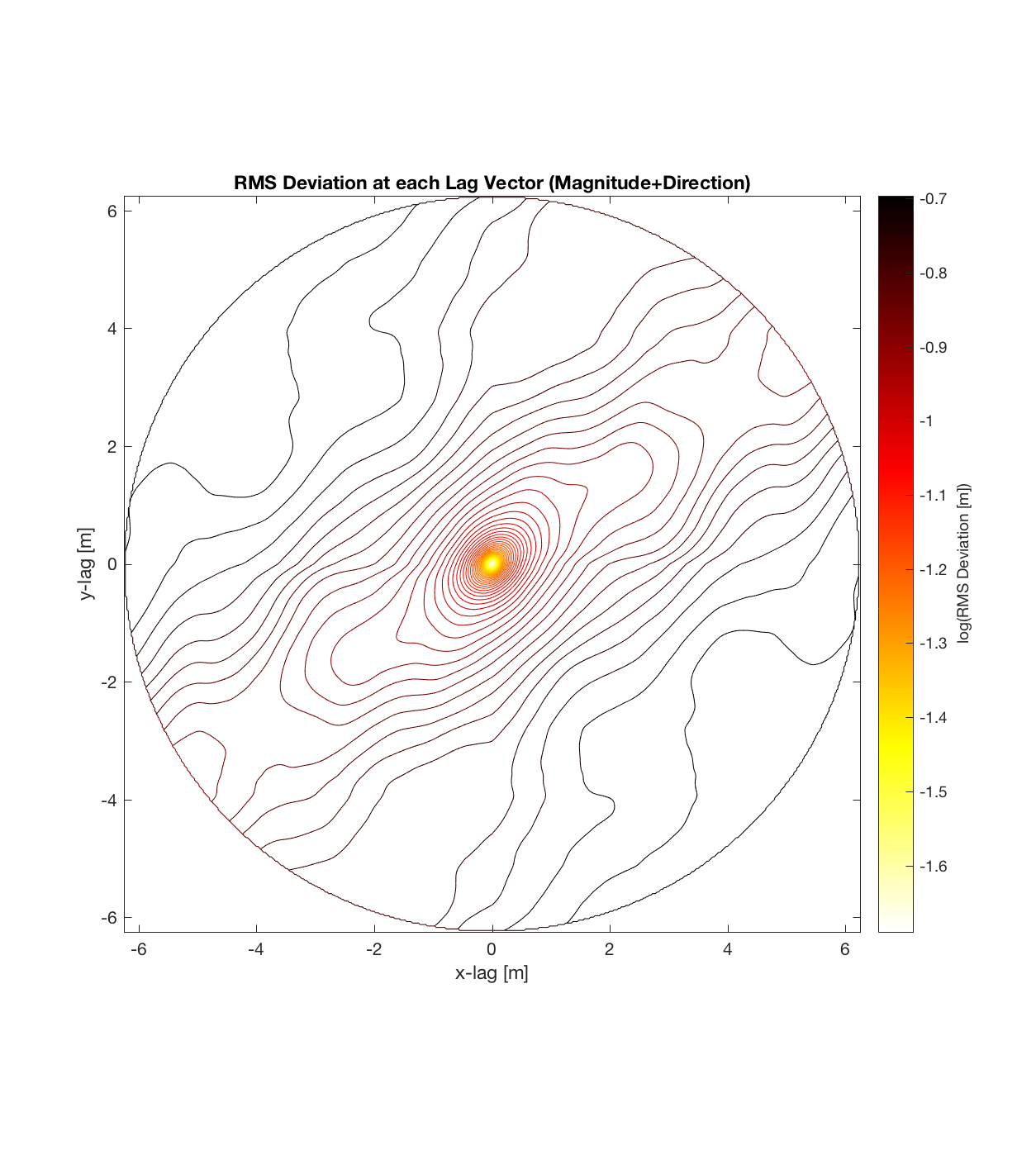
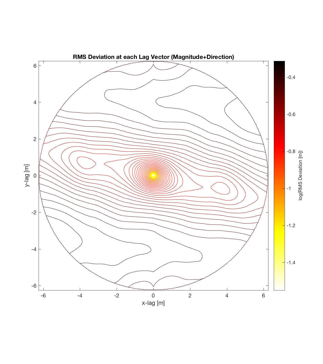
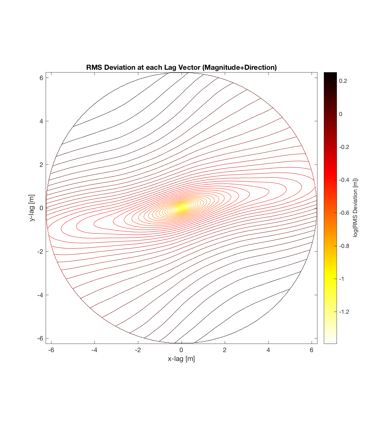
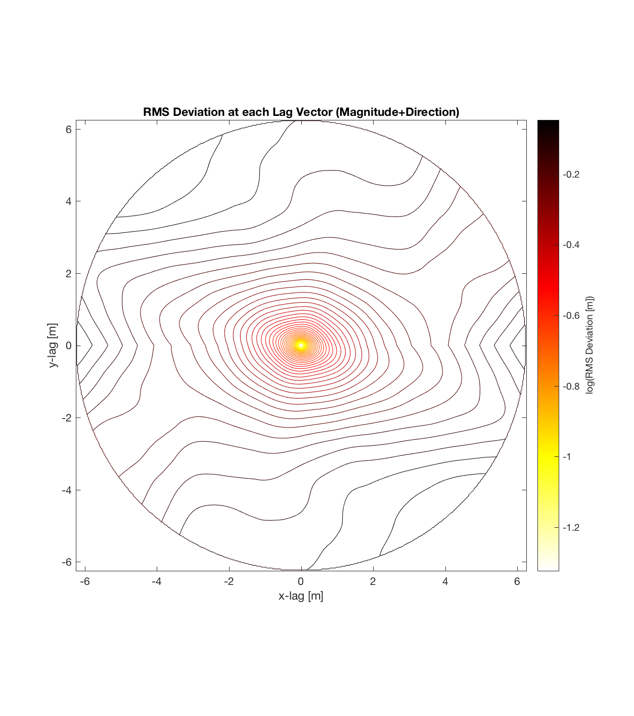
a) Can immediately visualize anisotropy (as given by a ‘roughness’ eclipse, that can be decomposed into 2 ‘principal axes of roughness’, corresponding to the directions in which the Hurst exponent is a maximum and minimum, respectively).
b) The final, contoured plot utilizes information from the entire spatial region; as opposed to the method of partitioning a DEM into cells of arbitrary size. This could be important because previously, the cell size could be affecting the ultimate roughness parameter values calculated, which would require a sensitivity analysis to account for. Effectively then, this approach treats the entire DEM as a single, large cell, maximizing the number of points available to sample given each lag vector. (Indeed, the sheer magnitude of the sample size is seen in the fact that each lag vector (ie. each point on the variorum) is now calculated on the basis of hundreds of thousands of points, such that the final contour plot of RMS Deviation over all lags is a result of hundreds of billions of calculations).
c) The process of converting elevations to RMS Deviation in ‘lag-space’ can be viewed somewhat analogously to the that of the (Discrete) Fourier Transform, which transforms data from the temporal/spatial domain to the frequency/wavelength domain – and I think that ‘lag’ is comparable to ‘wavelength’, in the approximate sense that both connote spatial scale. The only difference is then that whereas the DFT indicates the amplitude/power at each scale, the ‘Roughness Spectrum’ indicates the degree of roughness at each scale, while the spacing between the contours on this spectrum should be inversely proportional to the Hurst exponent (ie. closely spaced contours imply that RMS Deviation is changing rapidly with respect to scale, implying a relatively high Hurst exponent).
II) Results
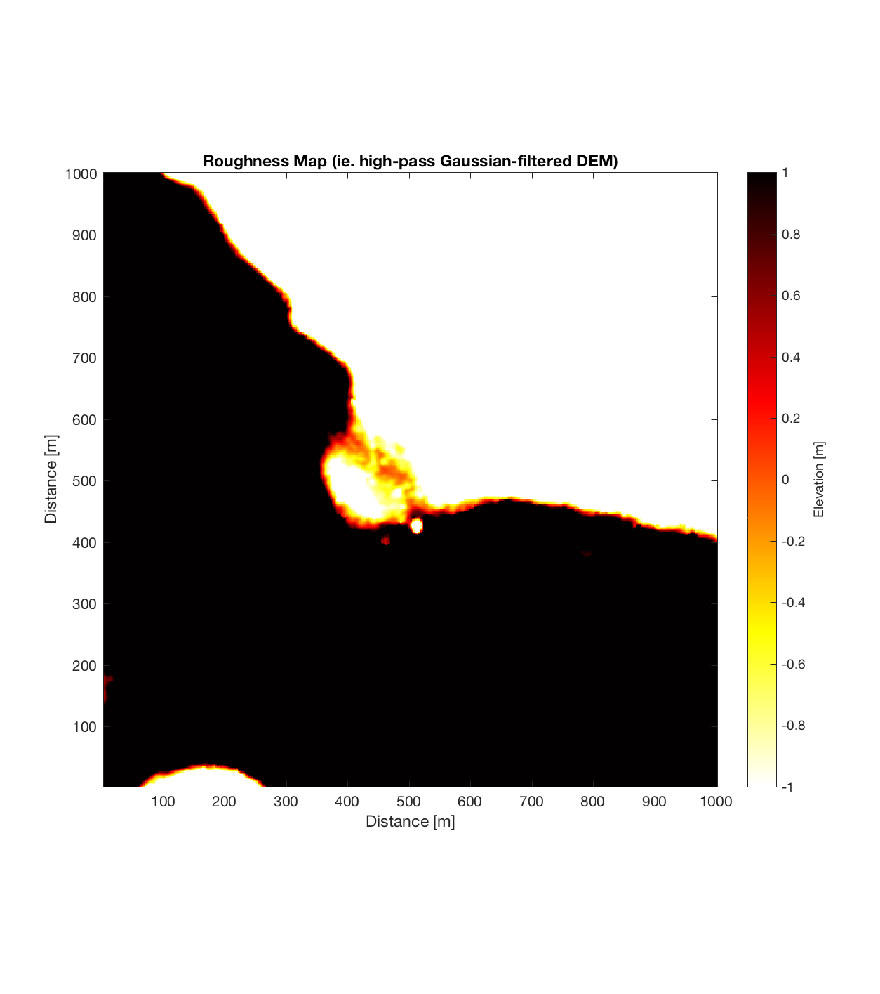
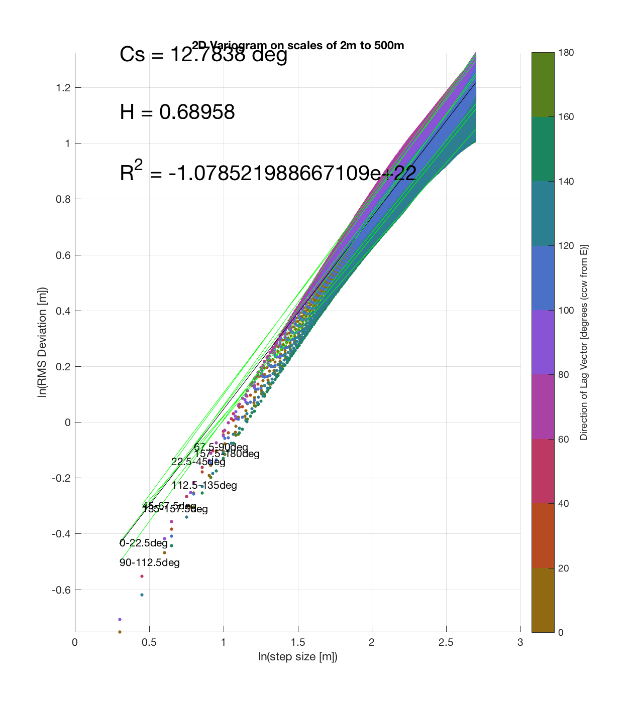
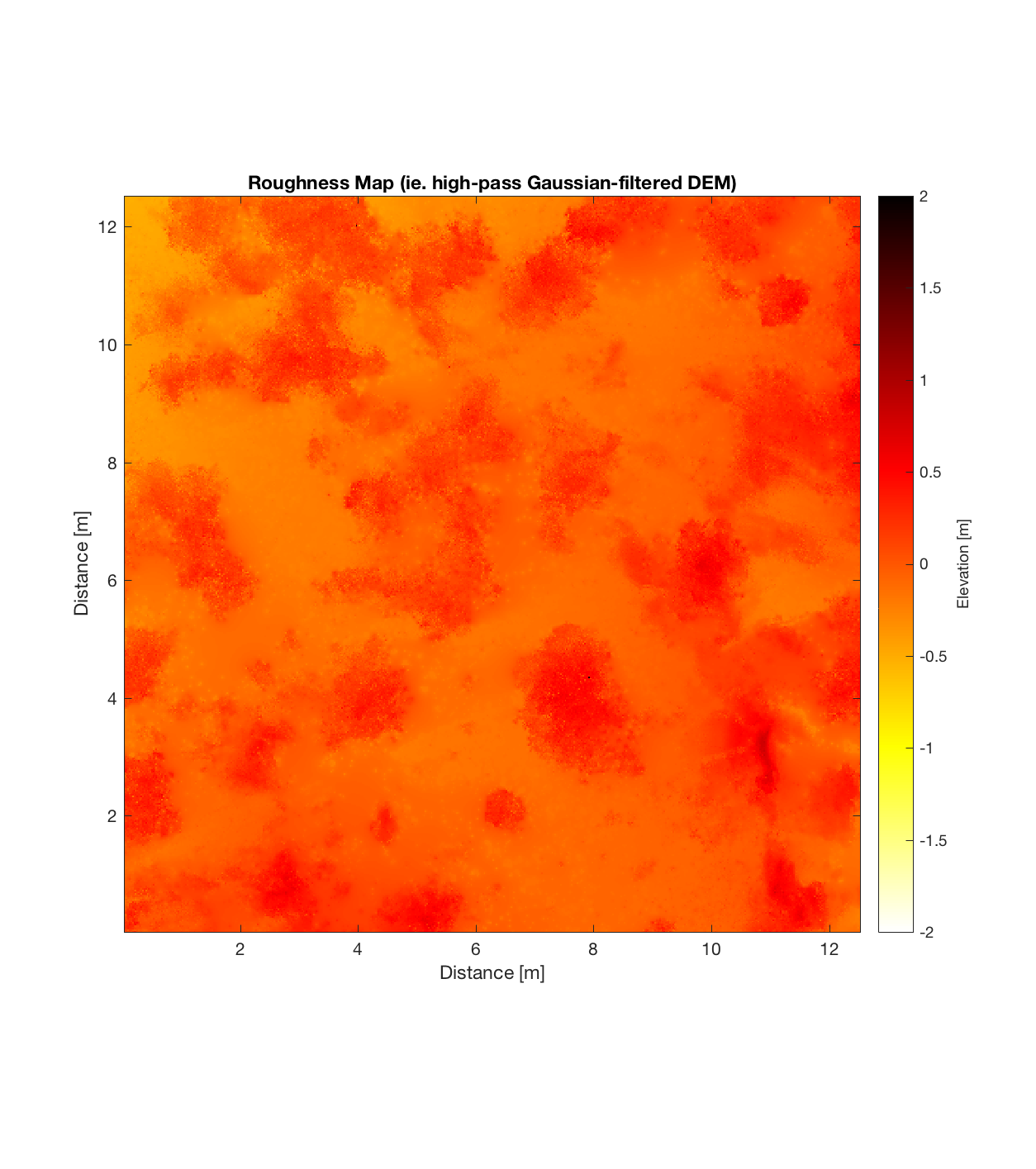
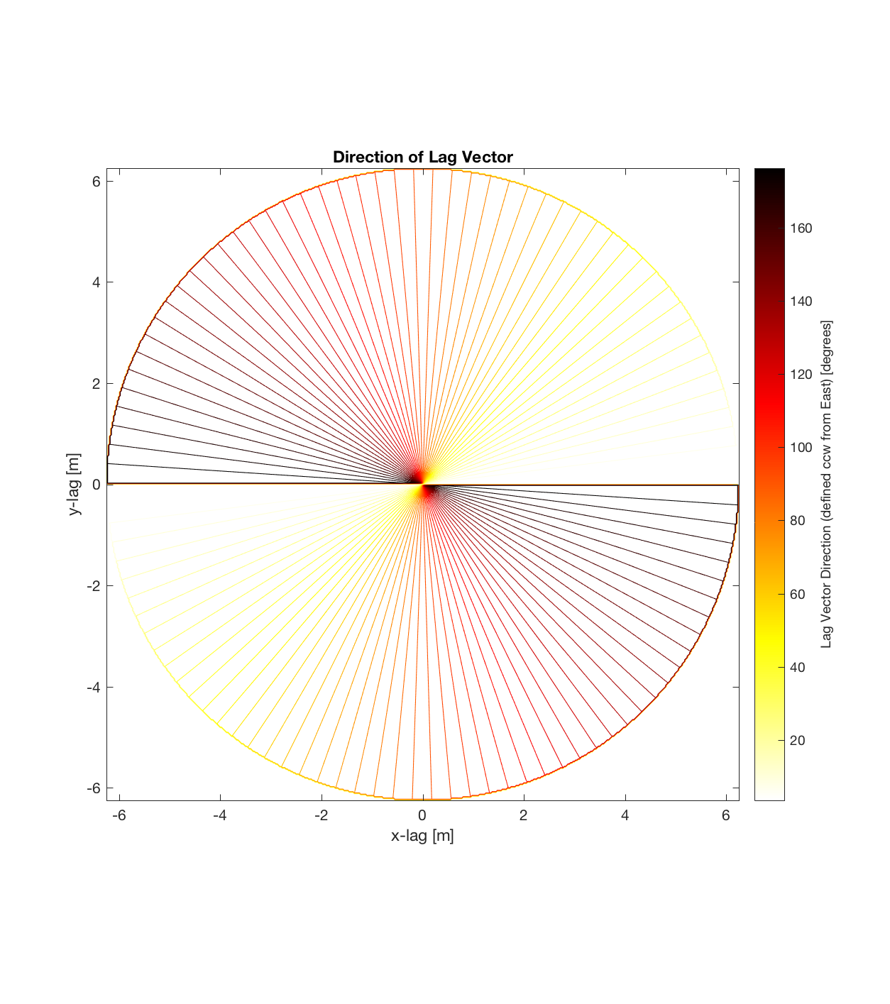
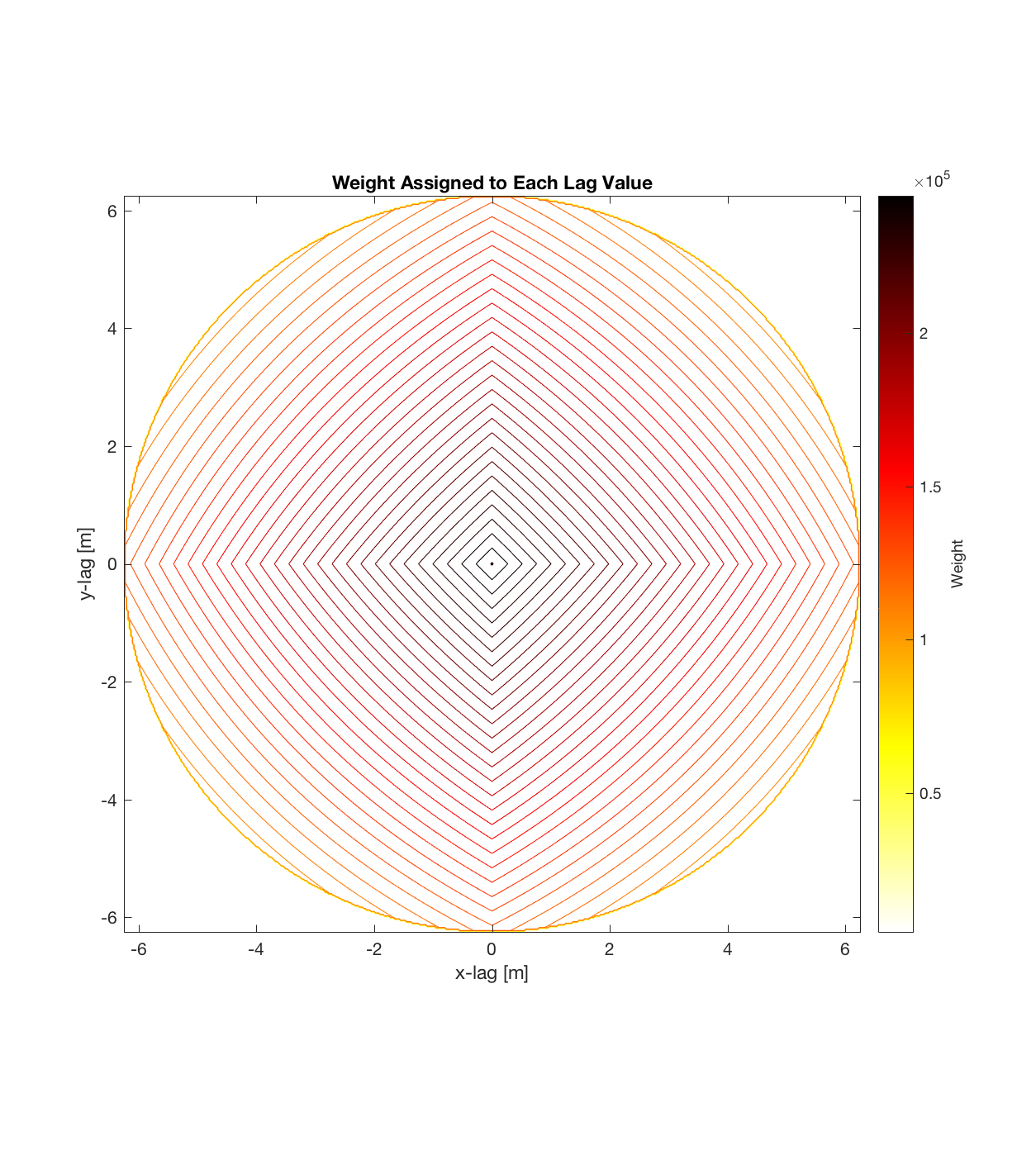
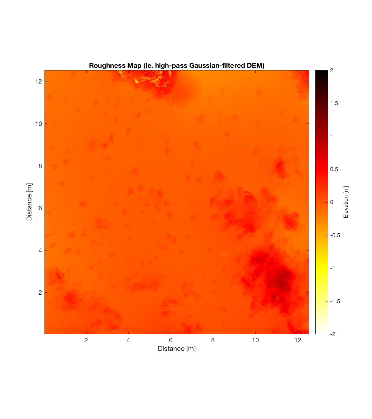
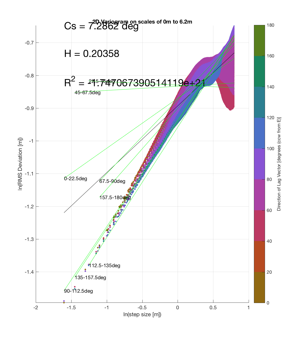
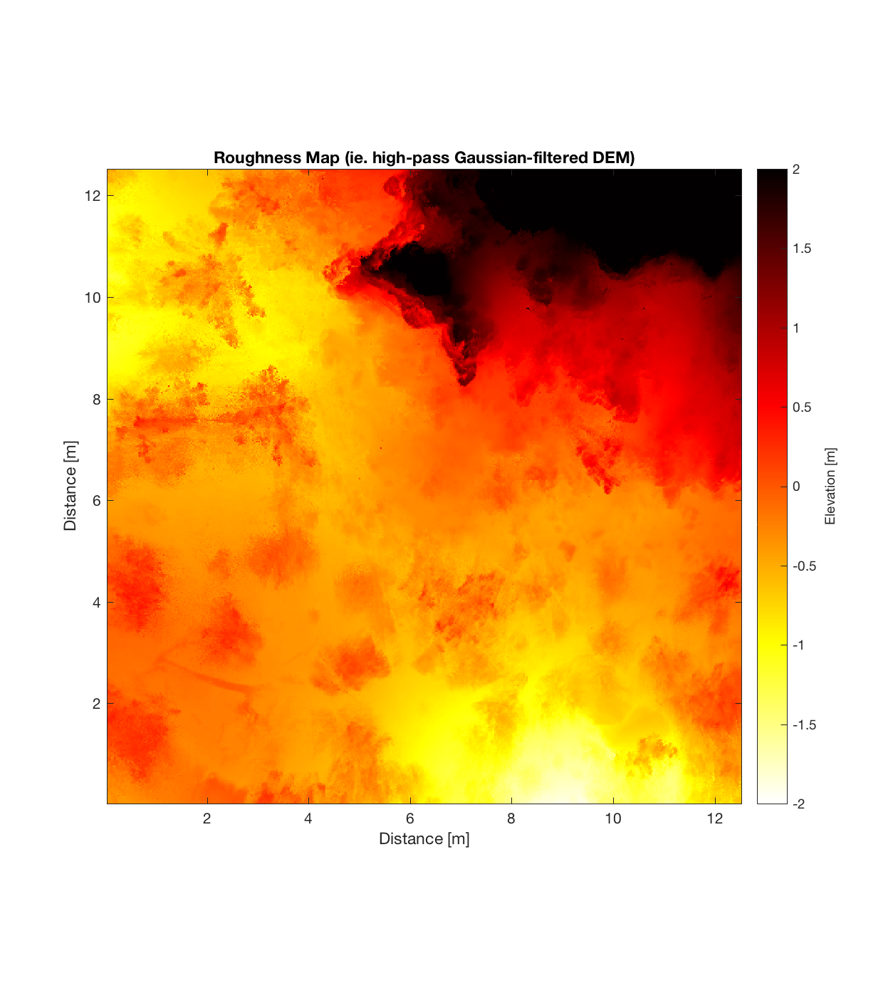
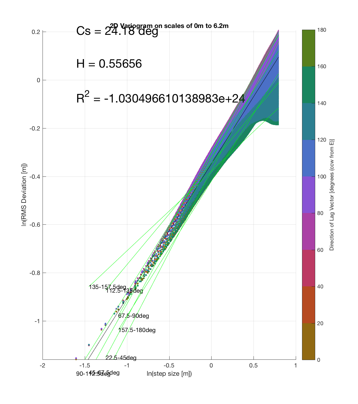
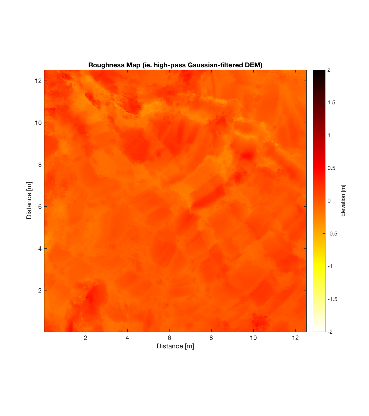
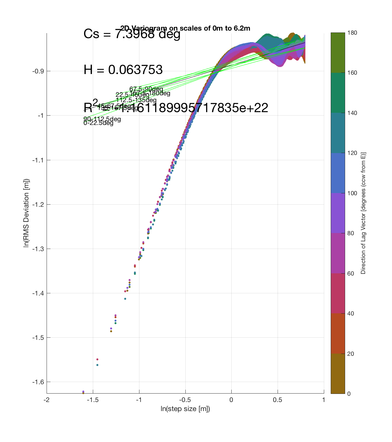
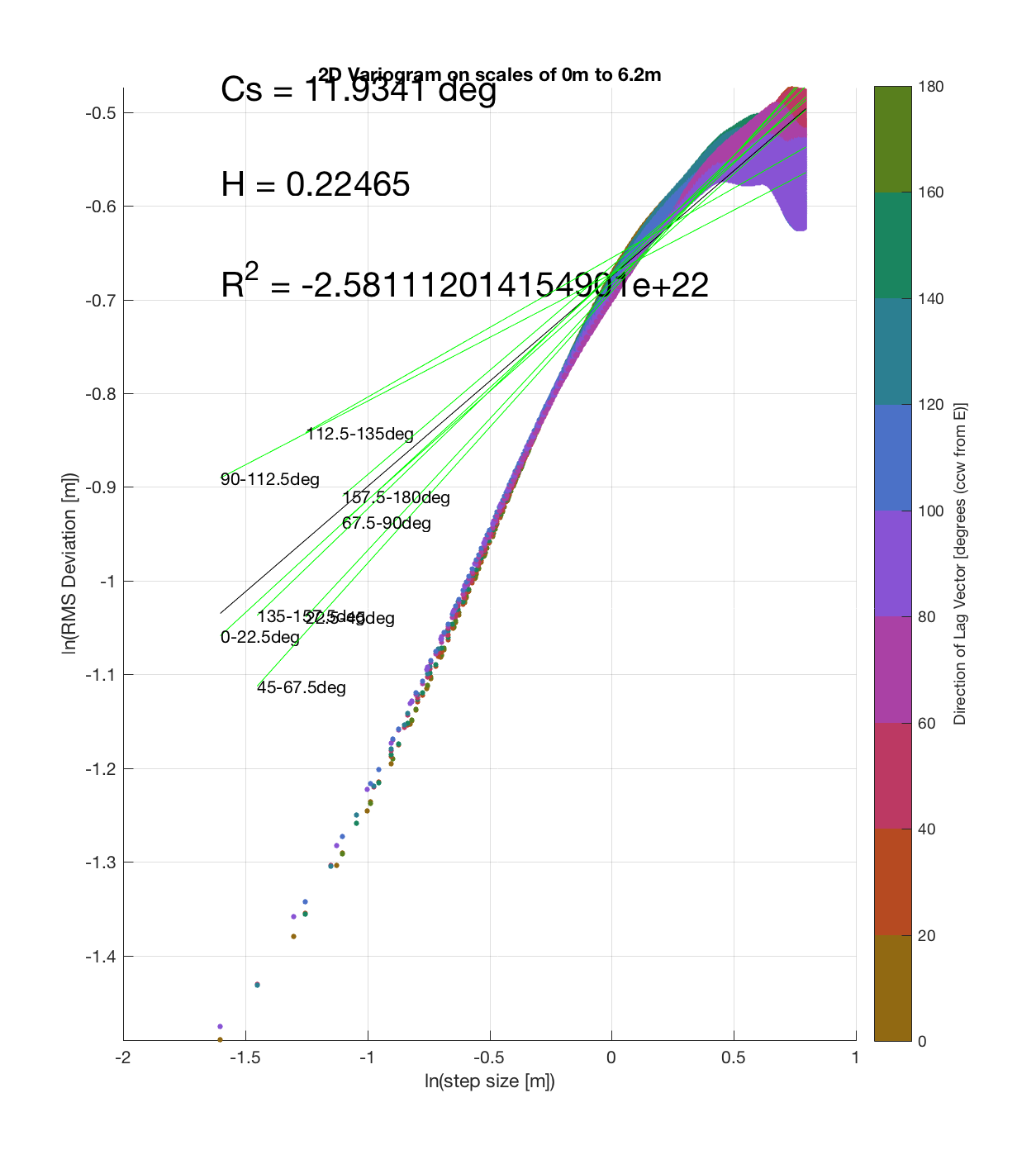
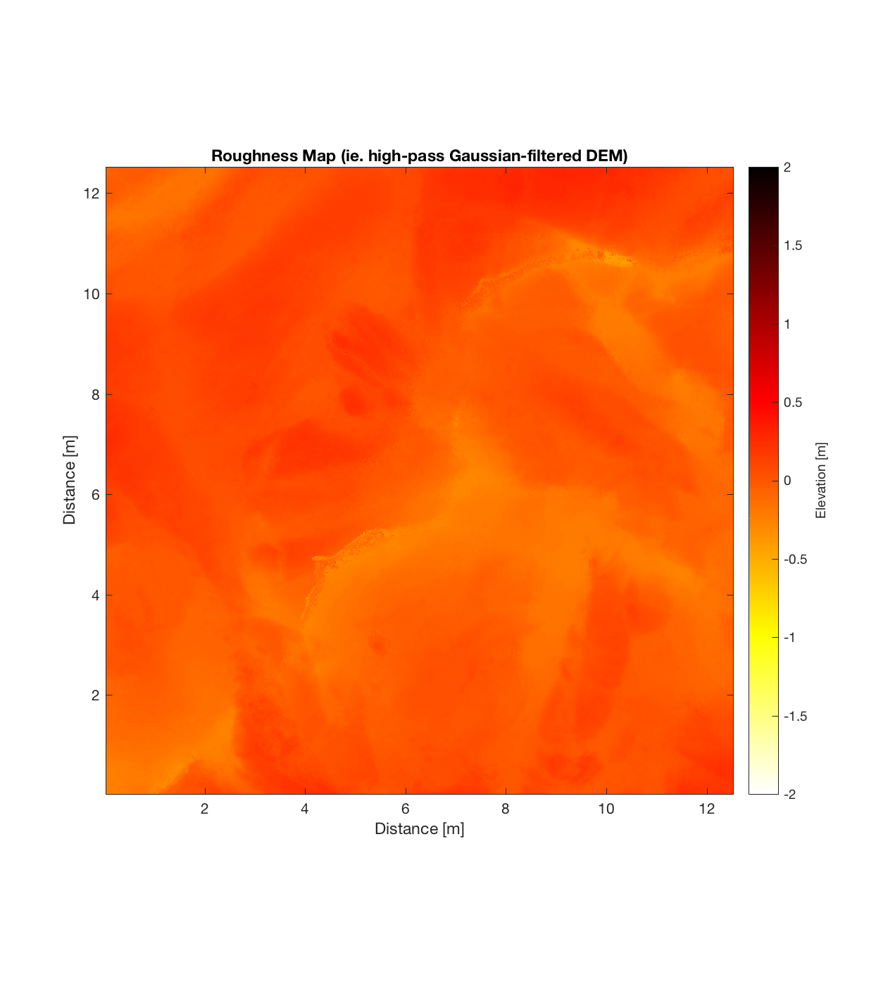
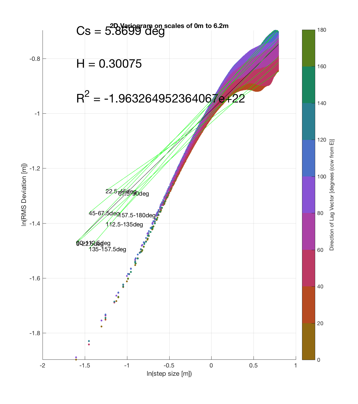
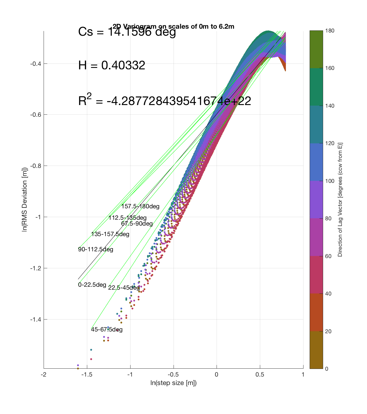
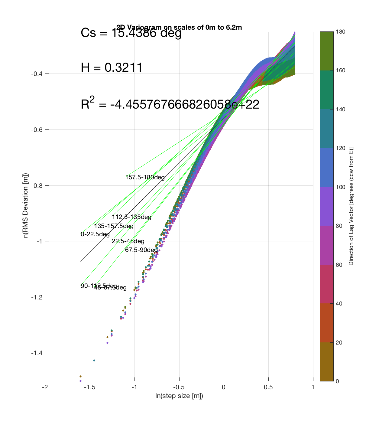
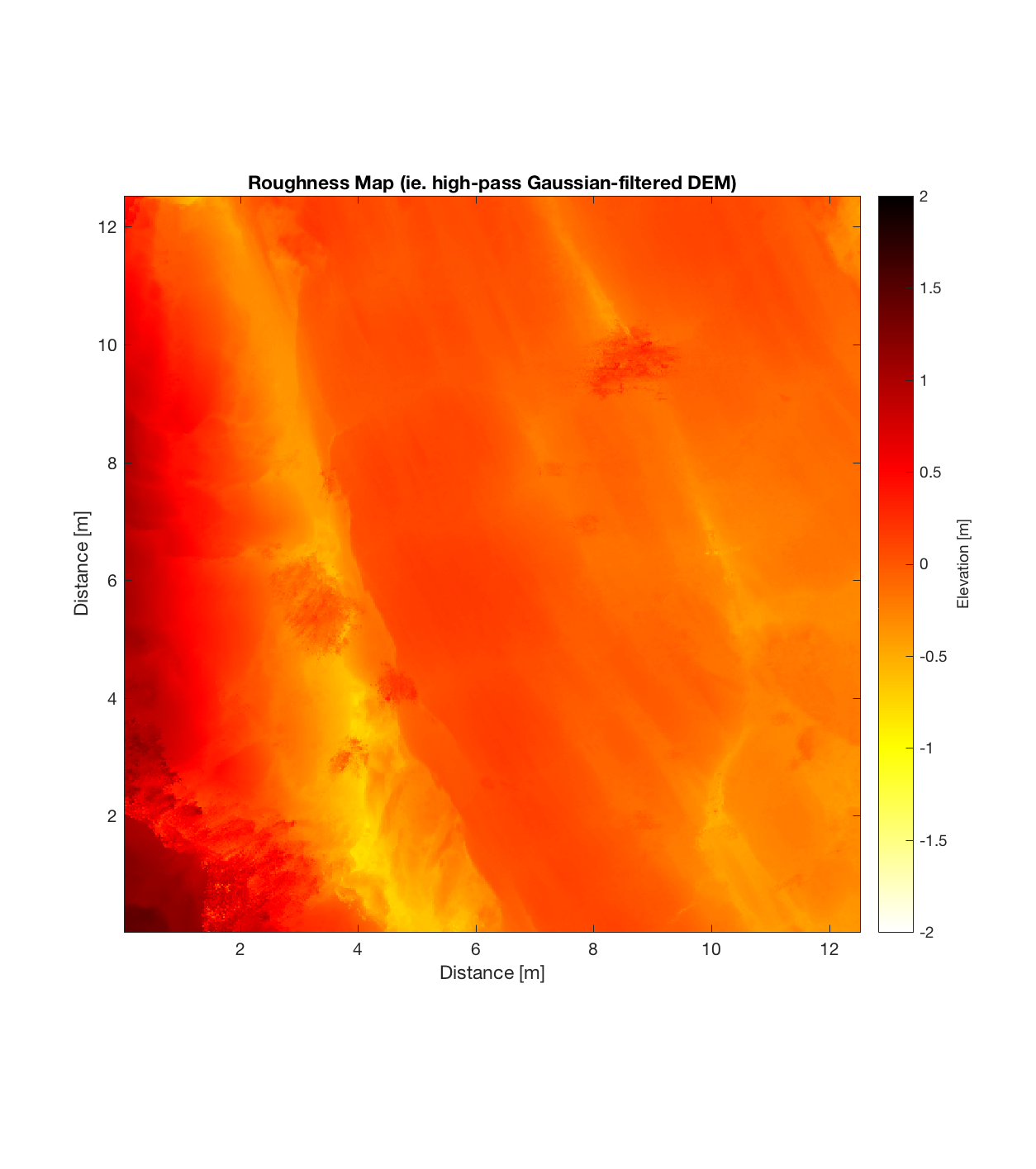
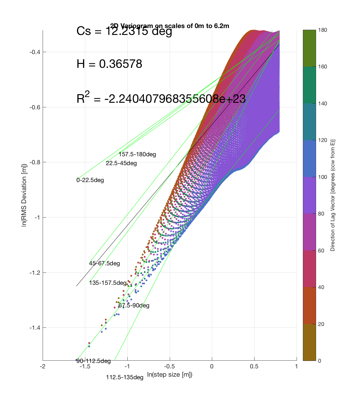
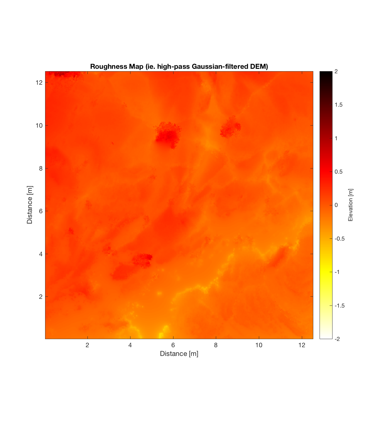
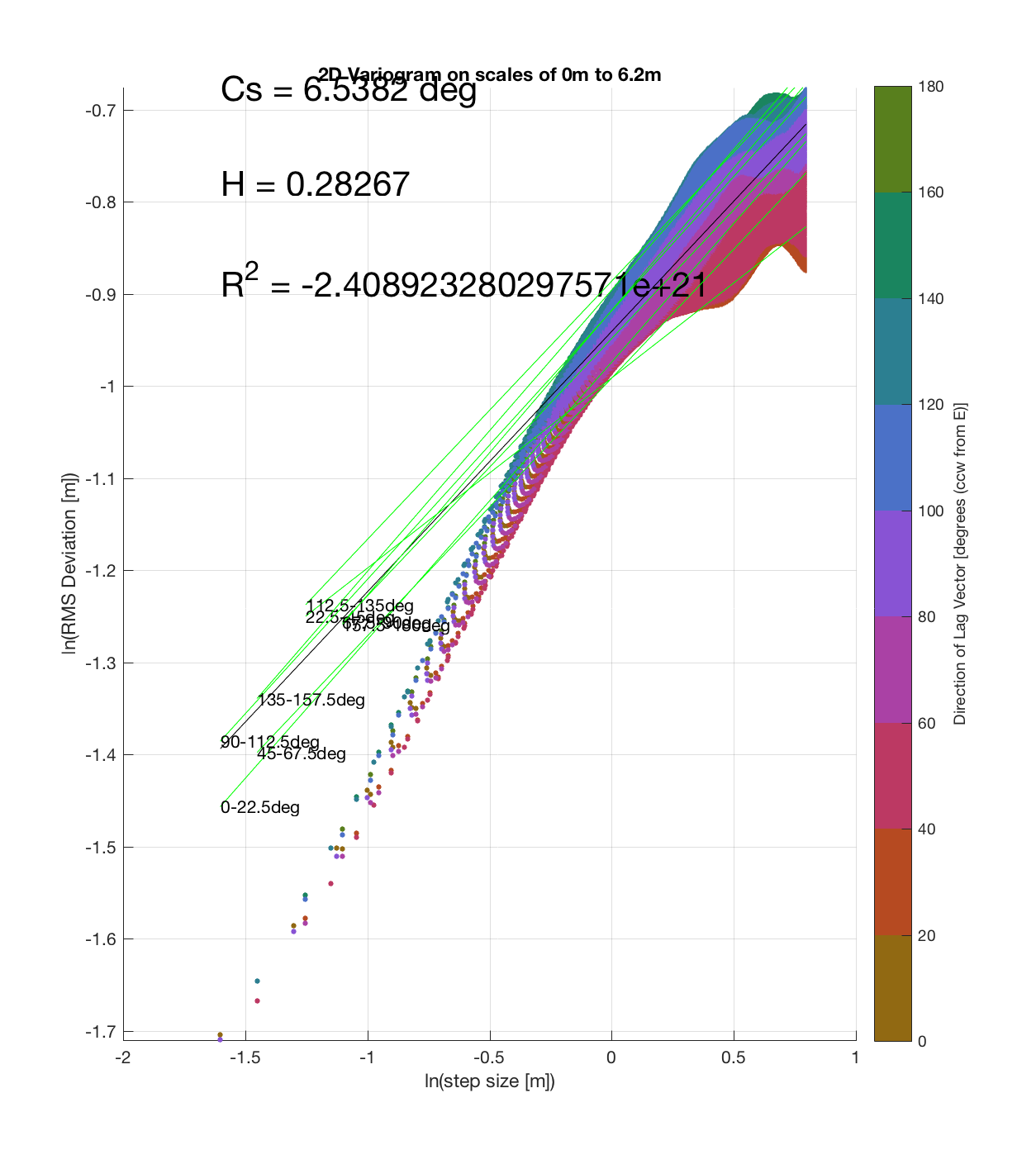
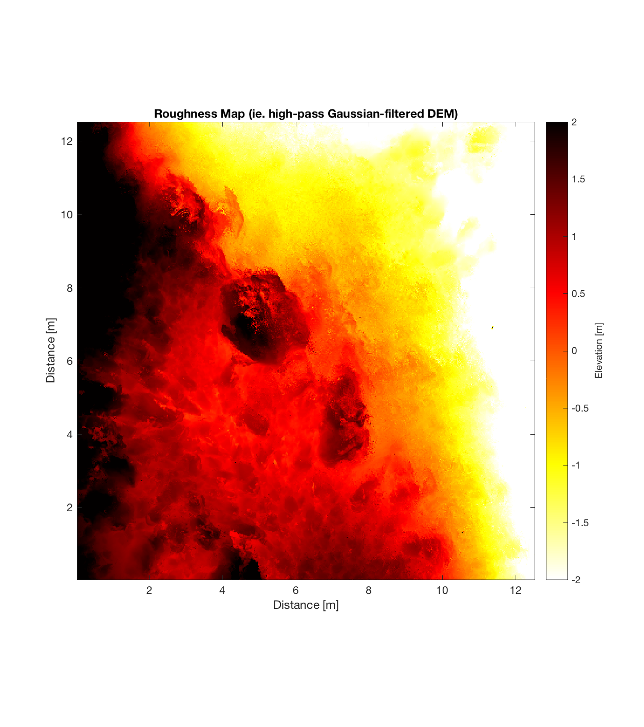
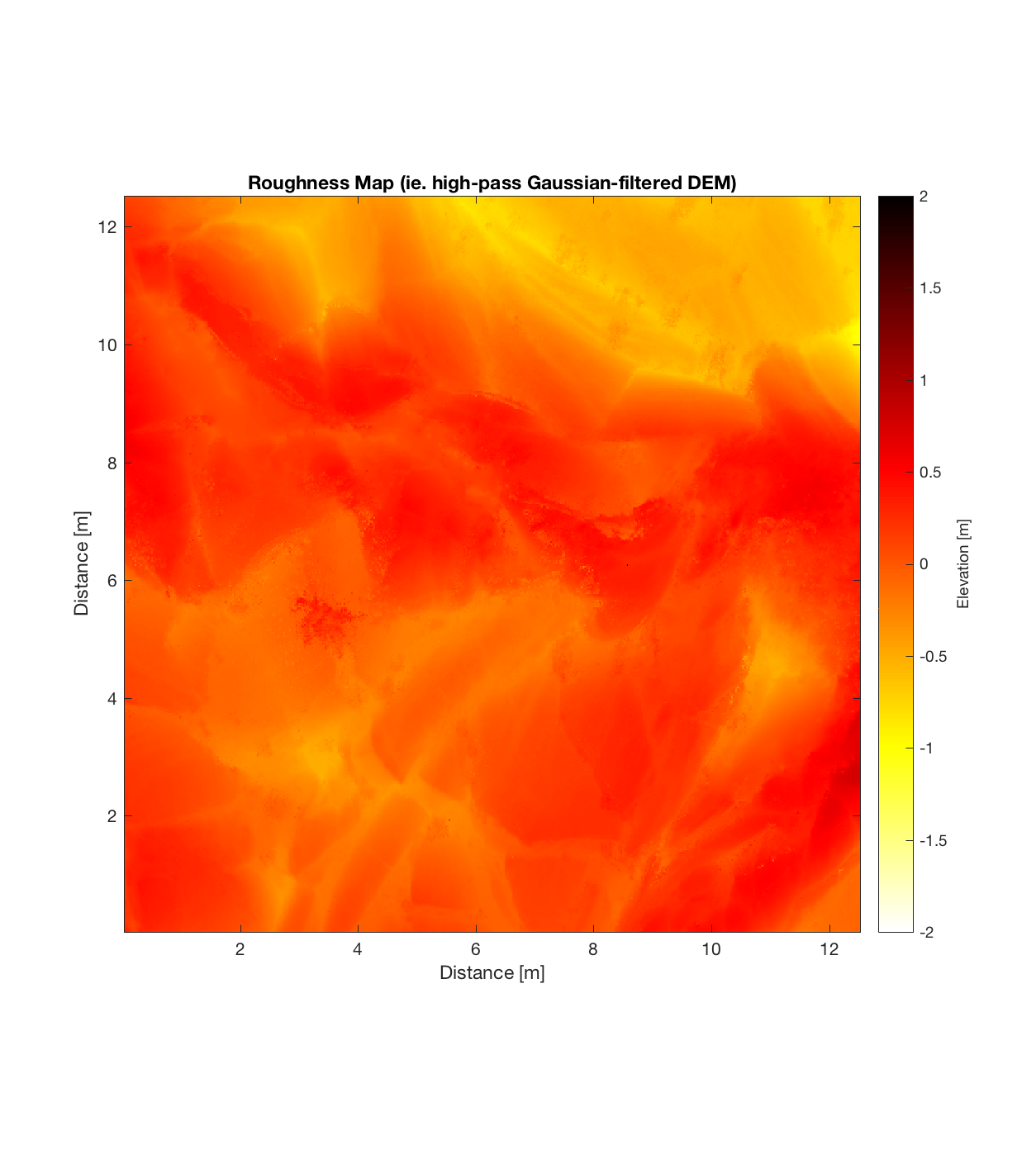
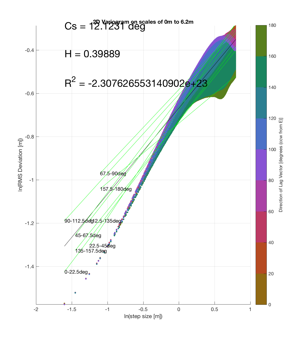
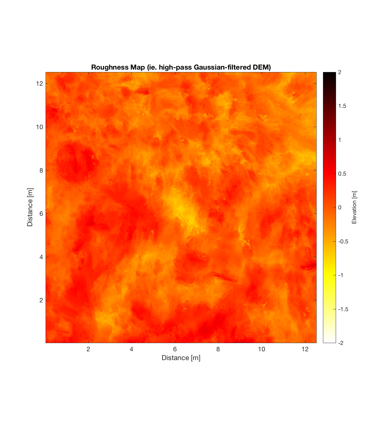
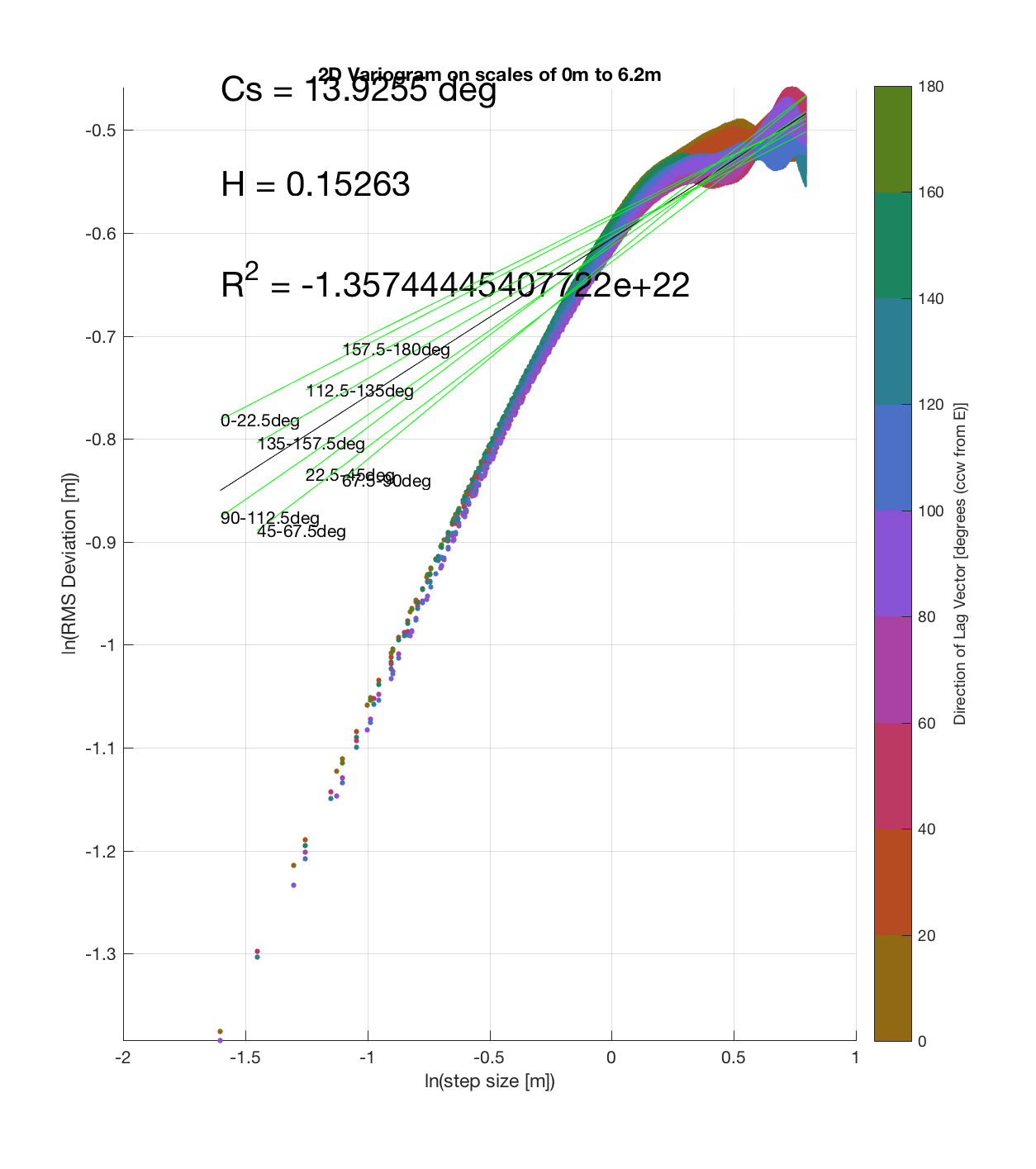
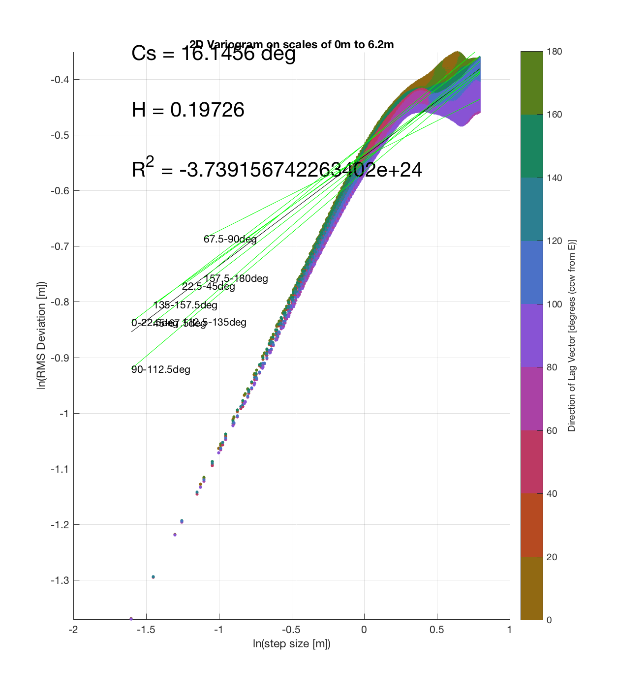
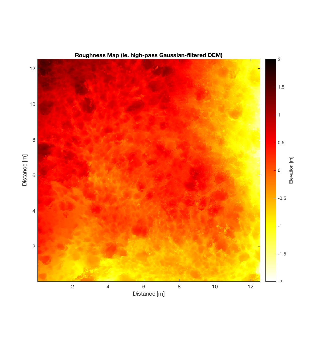
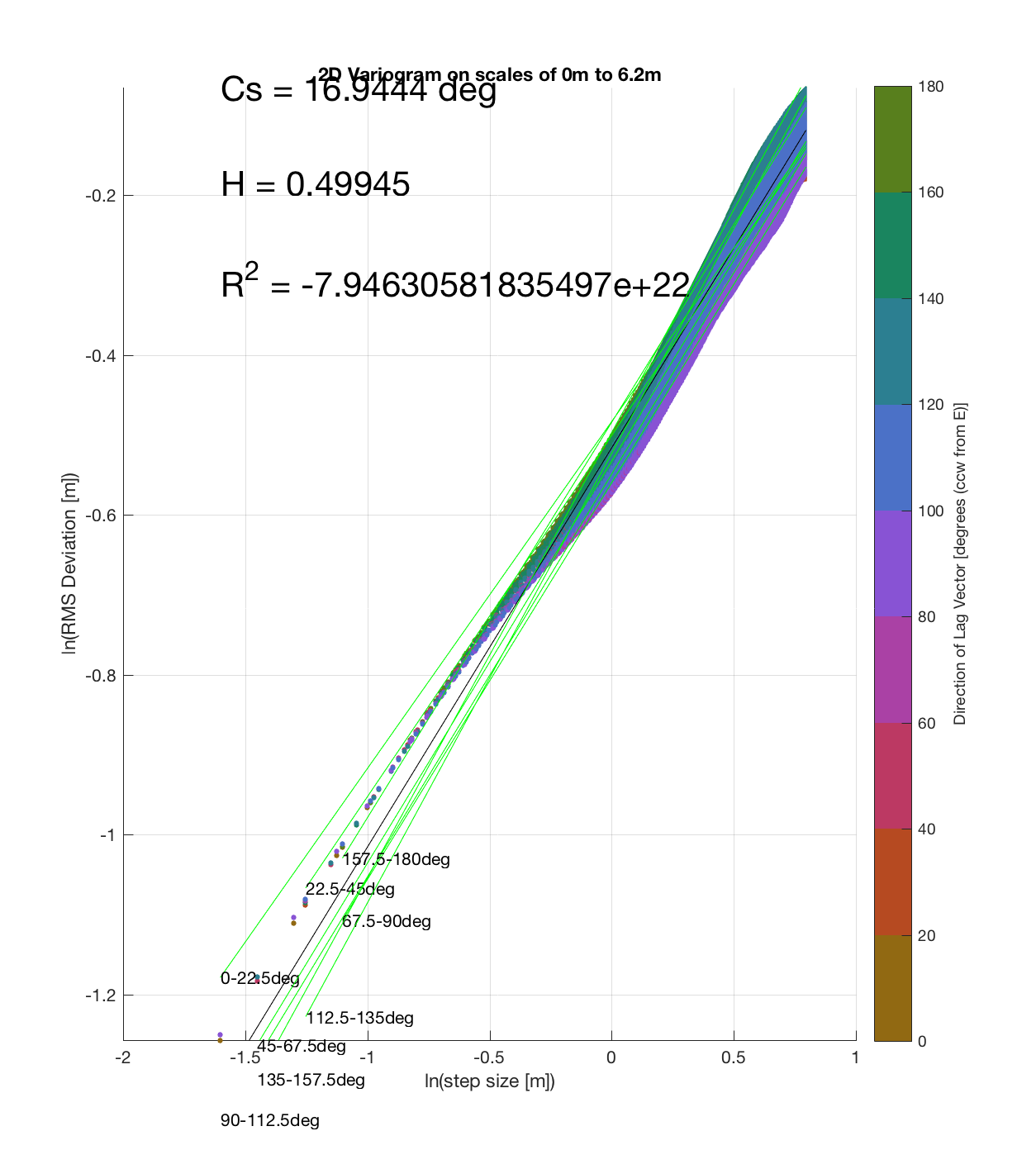
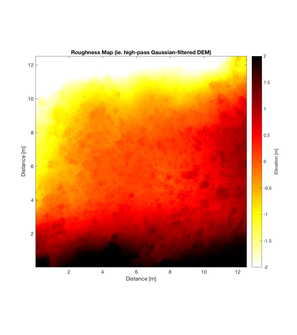
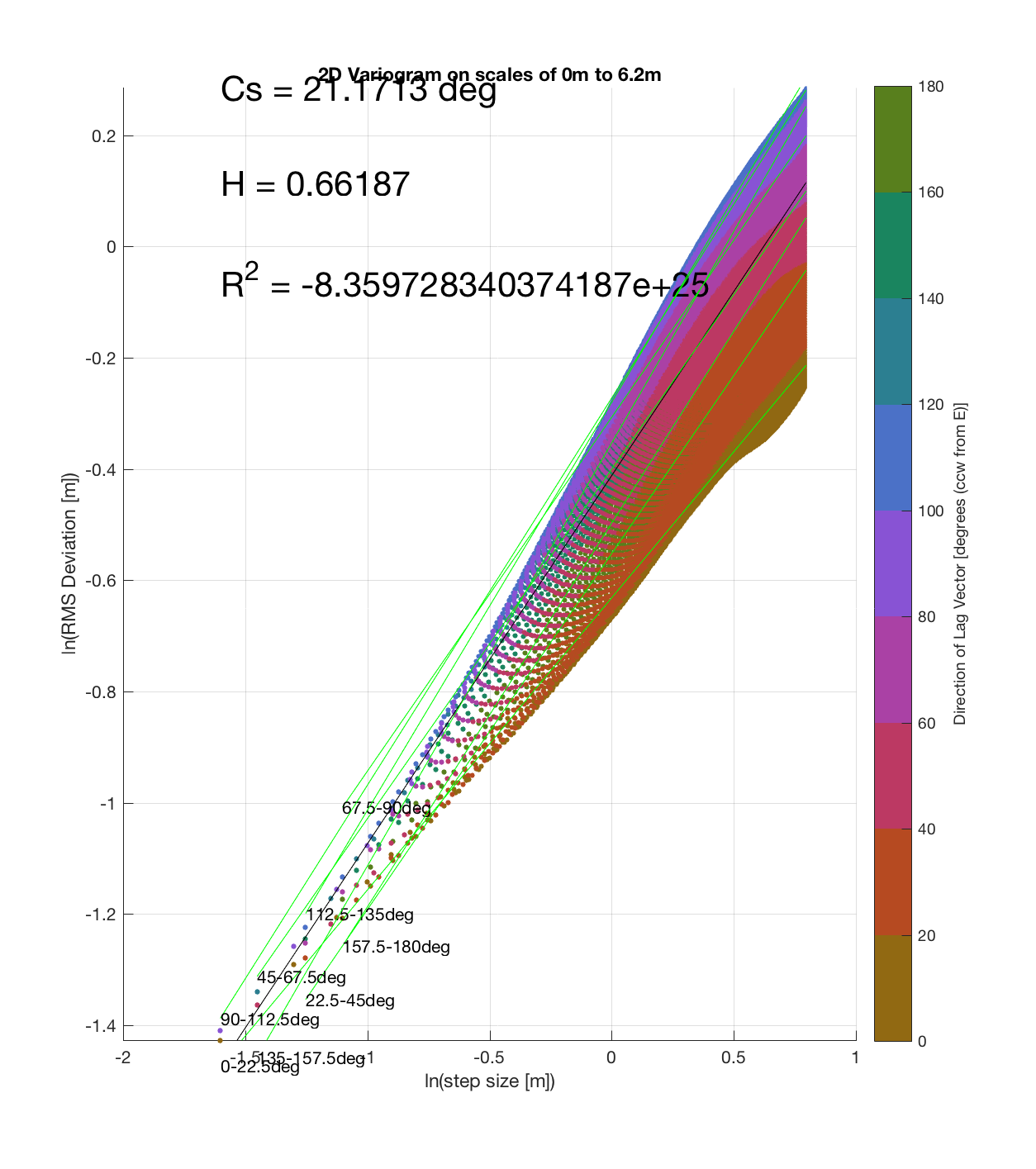
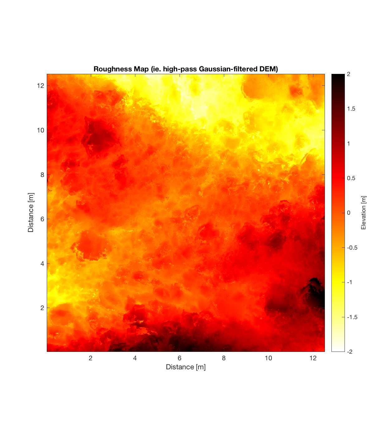
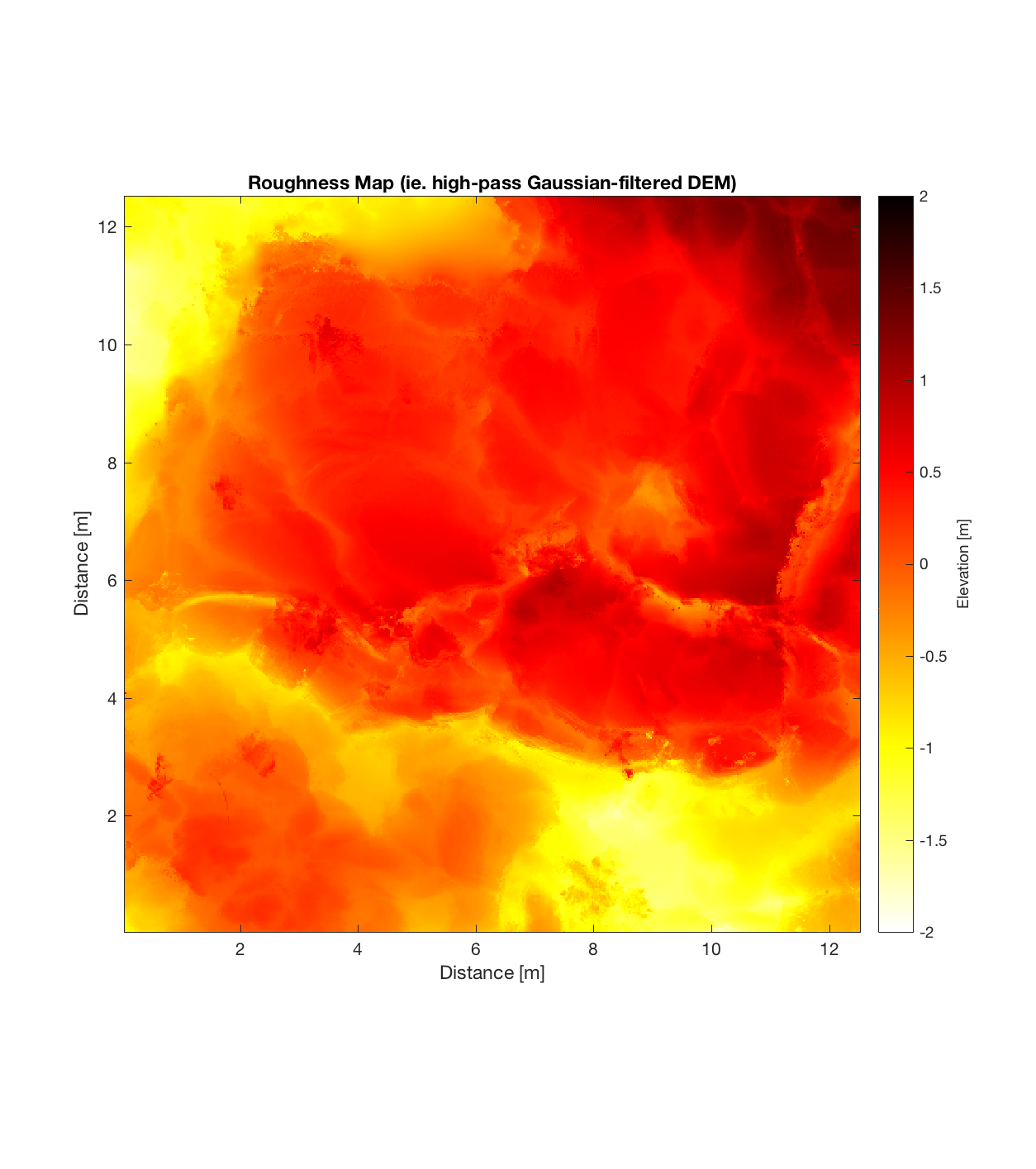
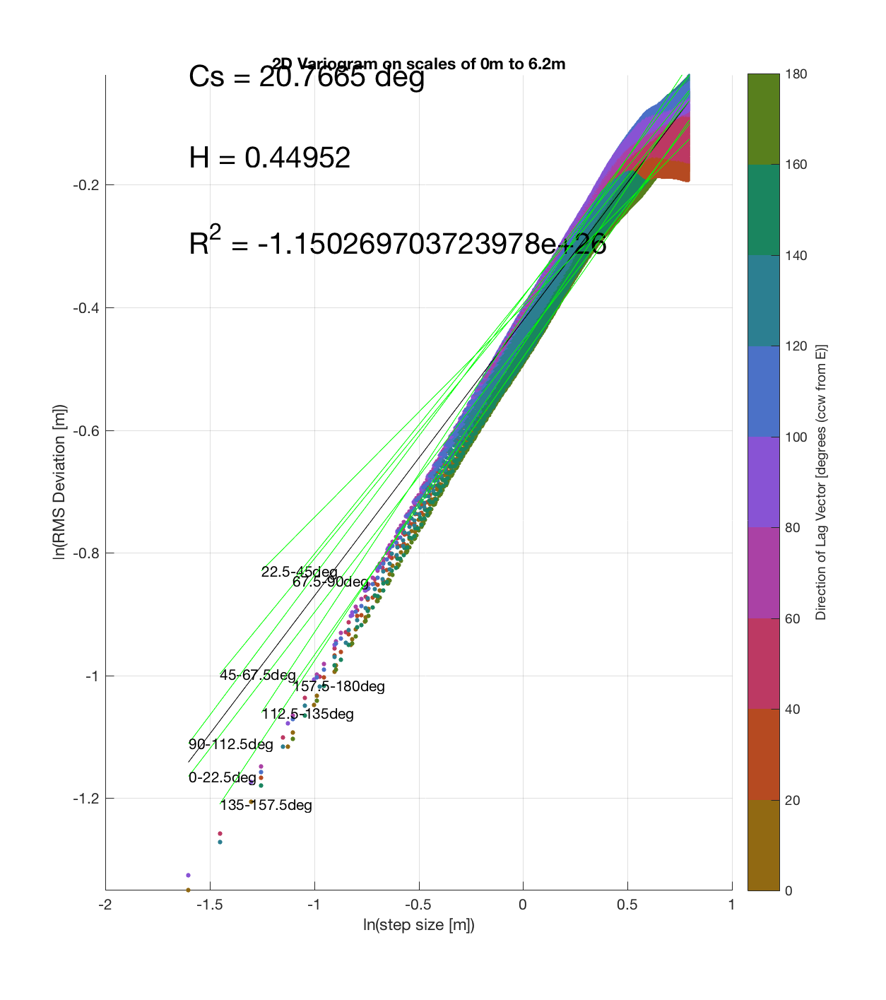
Below are plots for (almost all of) the COTM DEM’s from the 2016 field season (albeit high-pass filtered (‘de-trended’) by the 2D Gaussian Filter), where each is followed by a contour plot of the RMS Deviation with respect to lag vector (both magnitude and direction). Note that the positive y-lag region for each of these plots is symmetrical to the negative y-region (by a reflection in y-axis then a reflection in the x-axis), due to the fact that a lag of, for instance, <25, -5>cm is equivalent to a lag vector of <-25, 5>cm, or more generally, (a,b)=(-a,-b) for any constant a, b within the lag range. Accompanying the first set of plots, for Devil’s Orchard Walk 1, is a plot illustrating the convention employed for the lag vector direction, followed by a contour plot showing the number of points used to calculate the RMS Deviation for each lag vector.
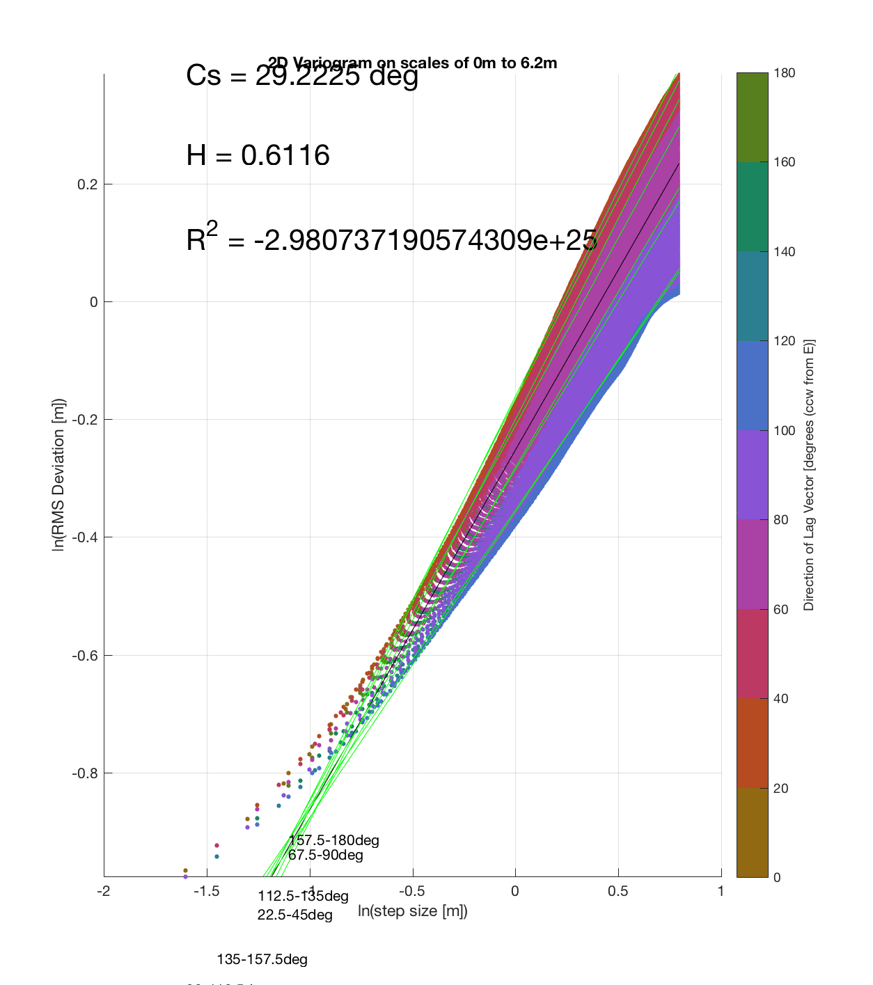
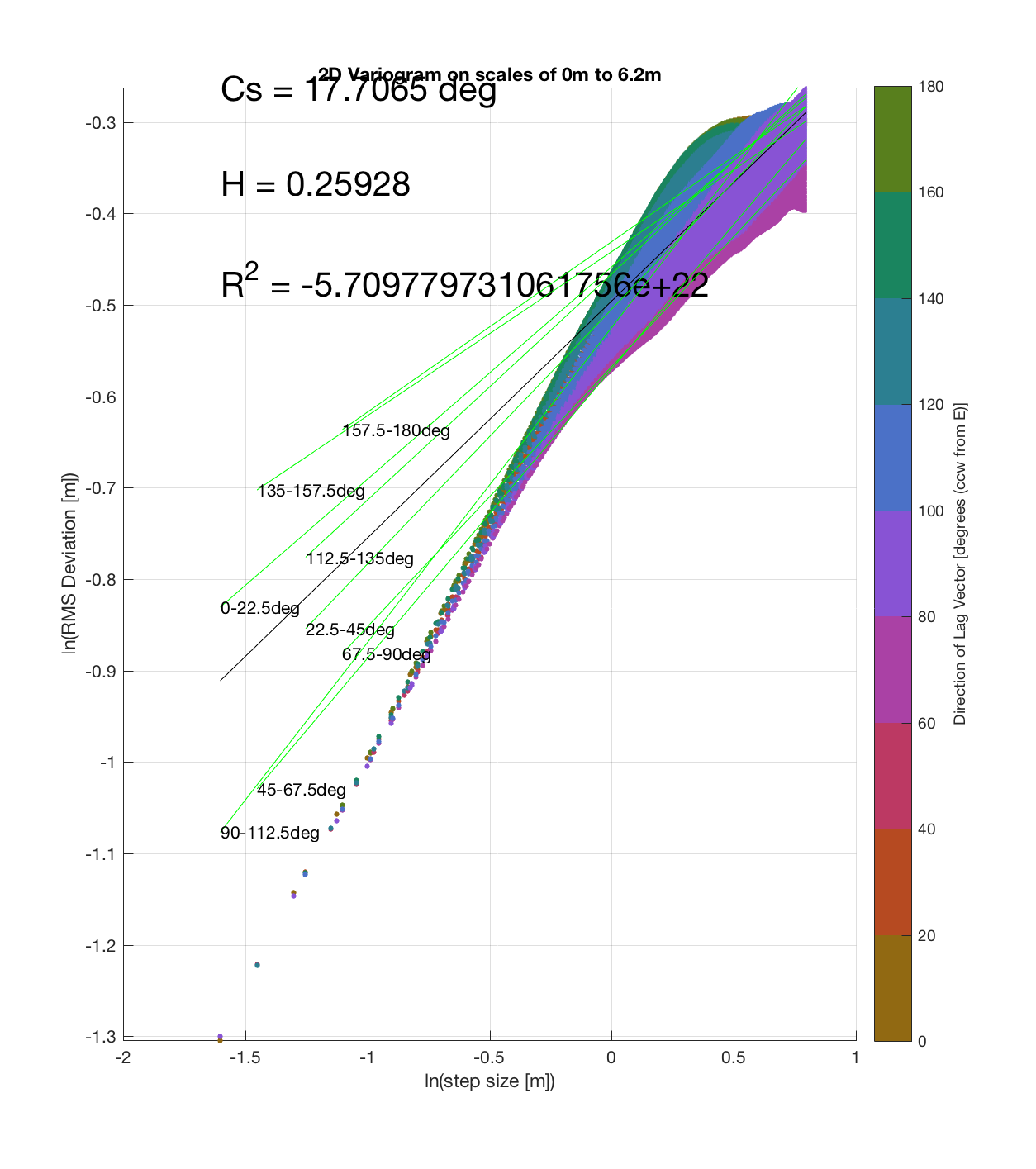
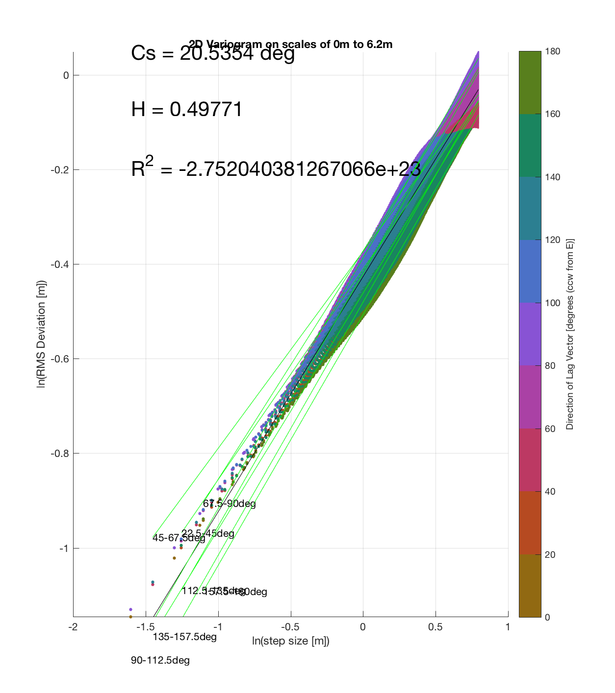
It should be noted that these RMS Deviation contour plots are more general visualizations of roughness at different scales than variograms because they are essentially 2D variograms – extracting a profile of the RMS Deviation along a straight slice through these contours gives a variogram in a particular direction. Furthermore, the significant anisotropy in most of these contour plot implies that an attempt to estimate the Hurst exponent from a single variogram that integrates RMS Deviations associated with lag vectors in all directions is flawed, due to the fact that Hurst exponent (proportional to contour spacing) often appears to vary substantially with respect to direction.
Devil’s Orchard Walk 1
Devil’s Orchard Walk 2
Devil’s Orchard Walk 3
Finger Flow
Highway Flow
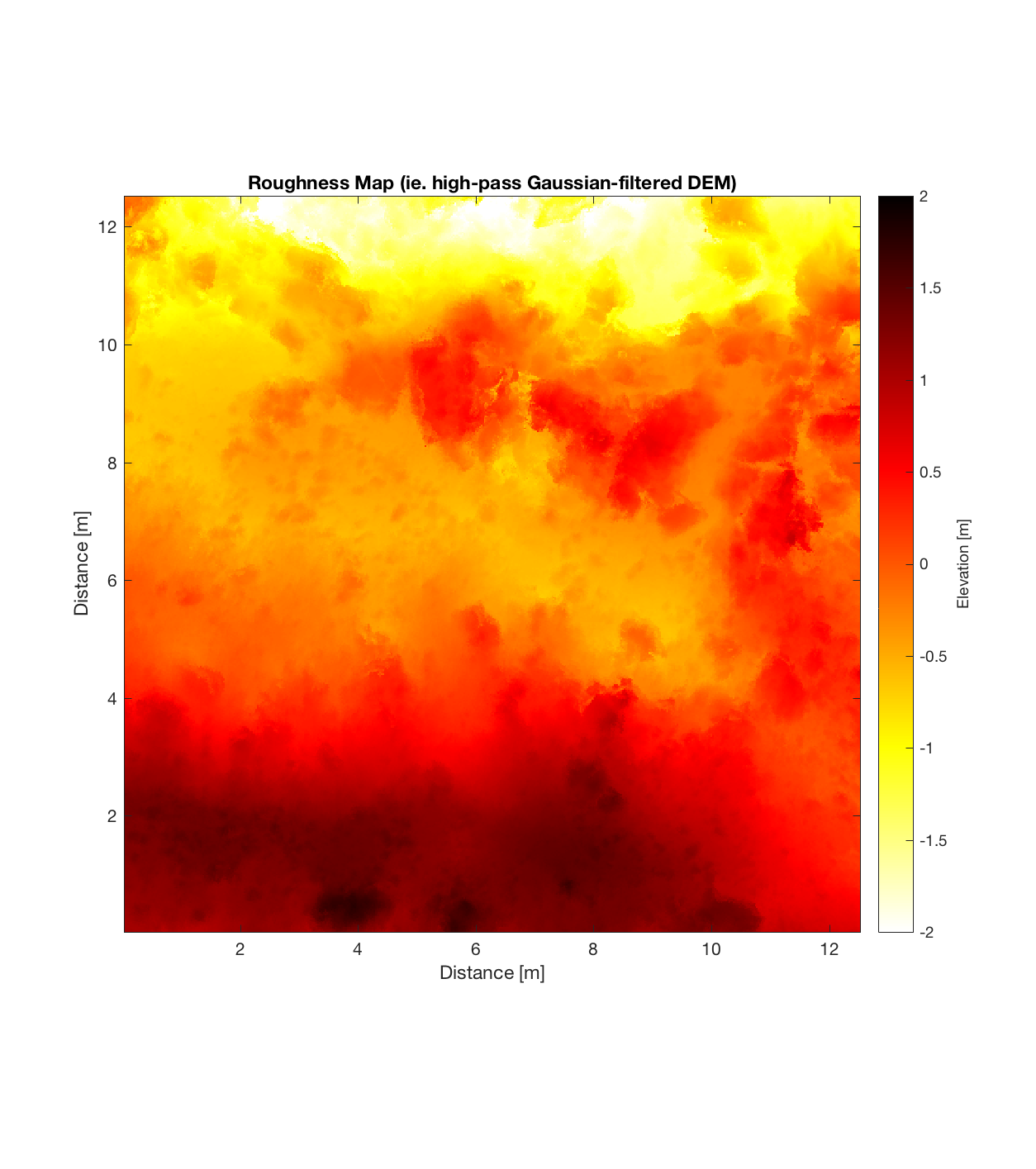
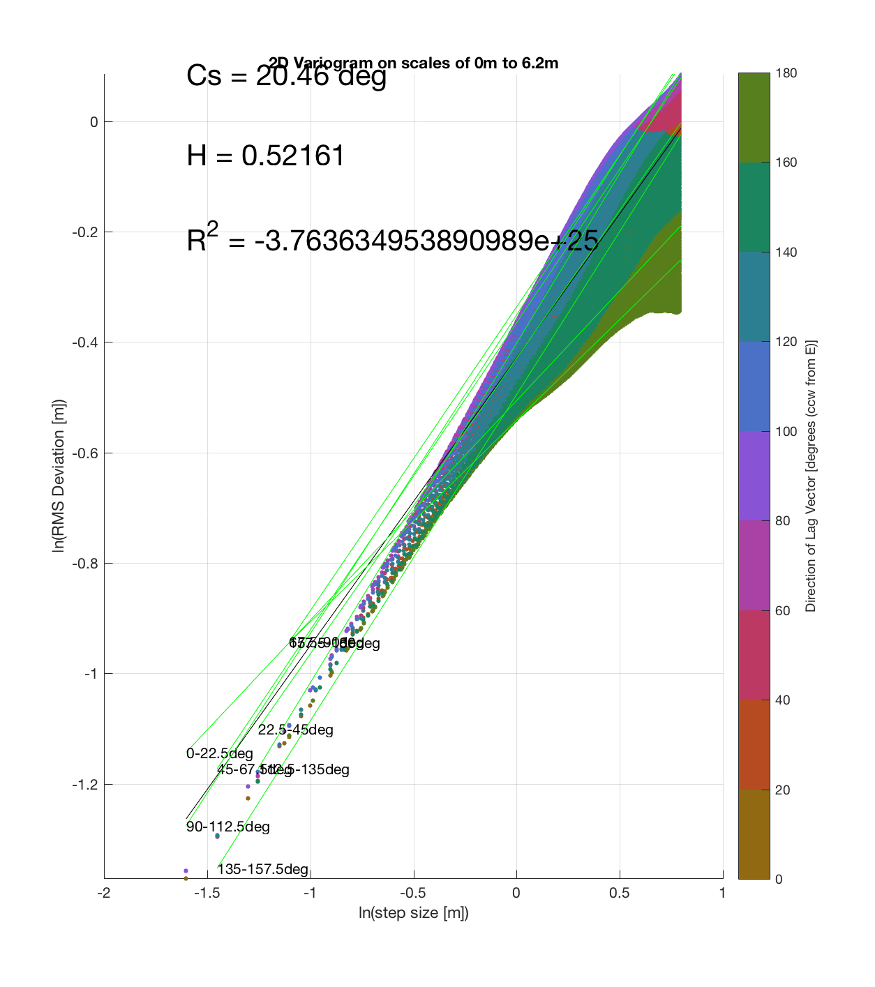
Indian Tunnel Top 1
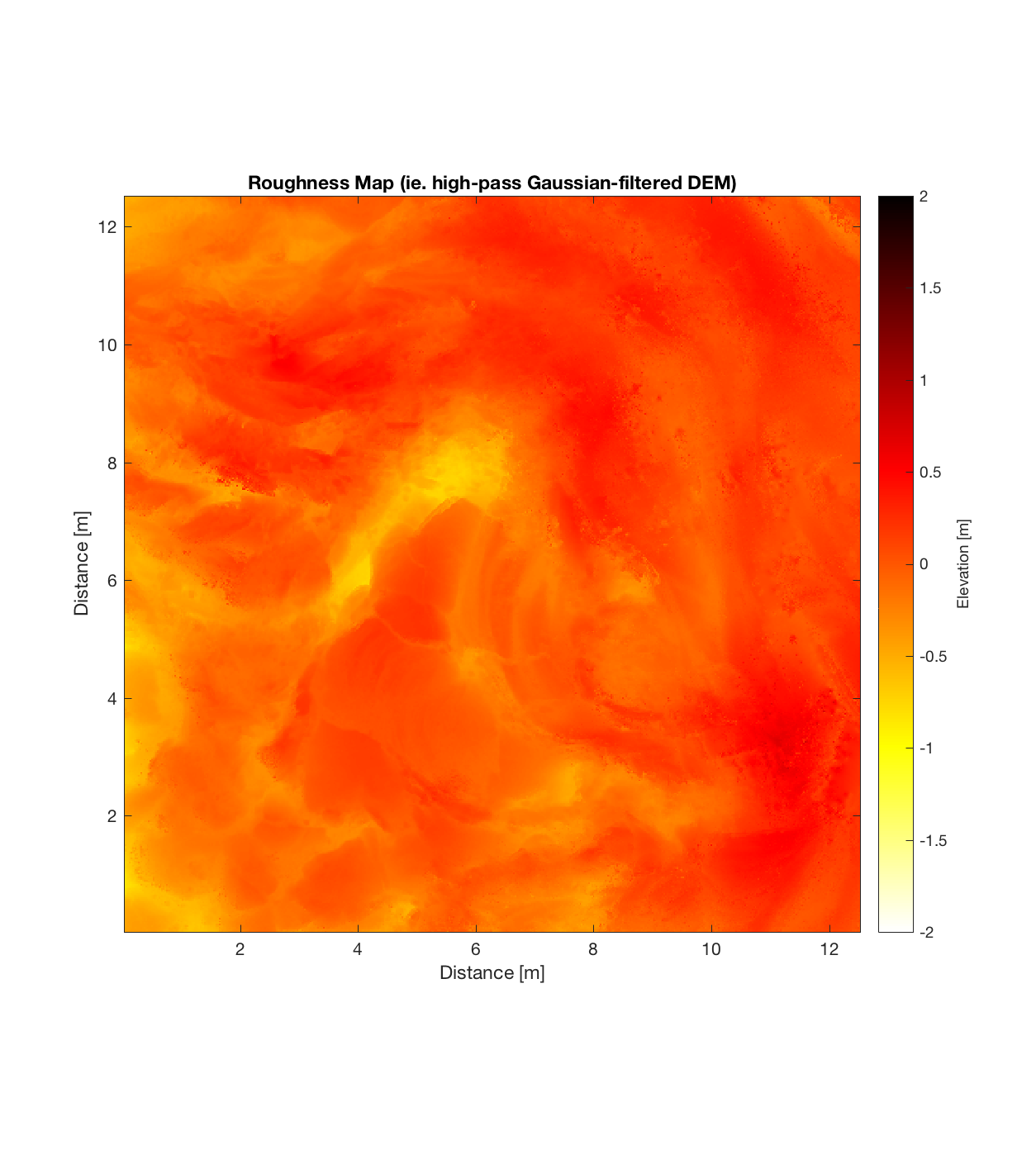

Indian Tunnel Top 2
Indian Tunnel Top 3
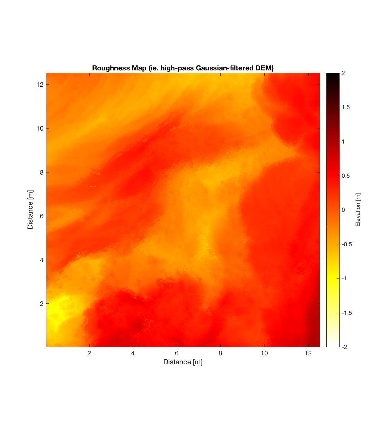
Indian Tunnel Top 4
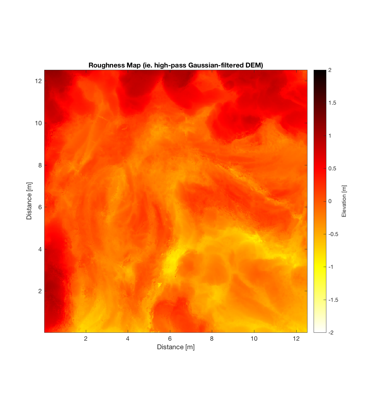
Lava Fall 1
Lava Fall 2
Orch Serr 1
Orch Serr 2
Orch Serr 3

Orch Serr 4
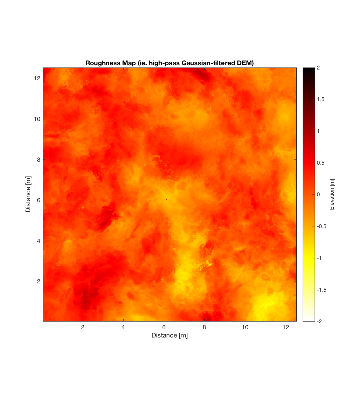
Rubbly Flow
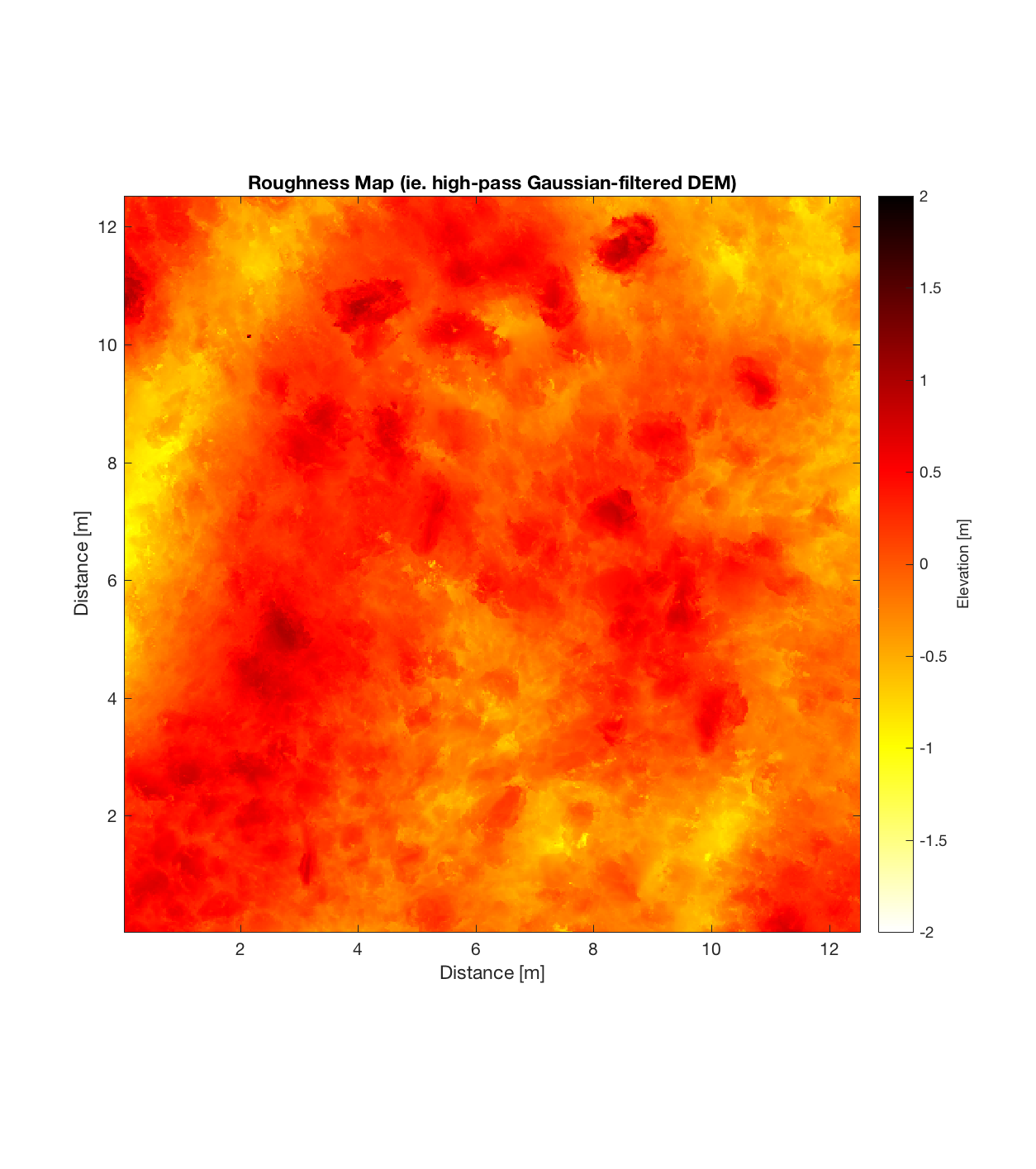
Serrate 2
Serrate 3
Serrate 4
Serrate 5
Spatter cone 1
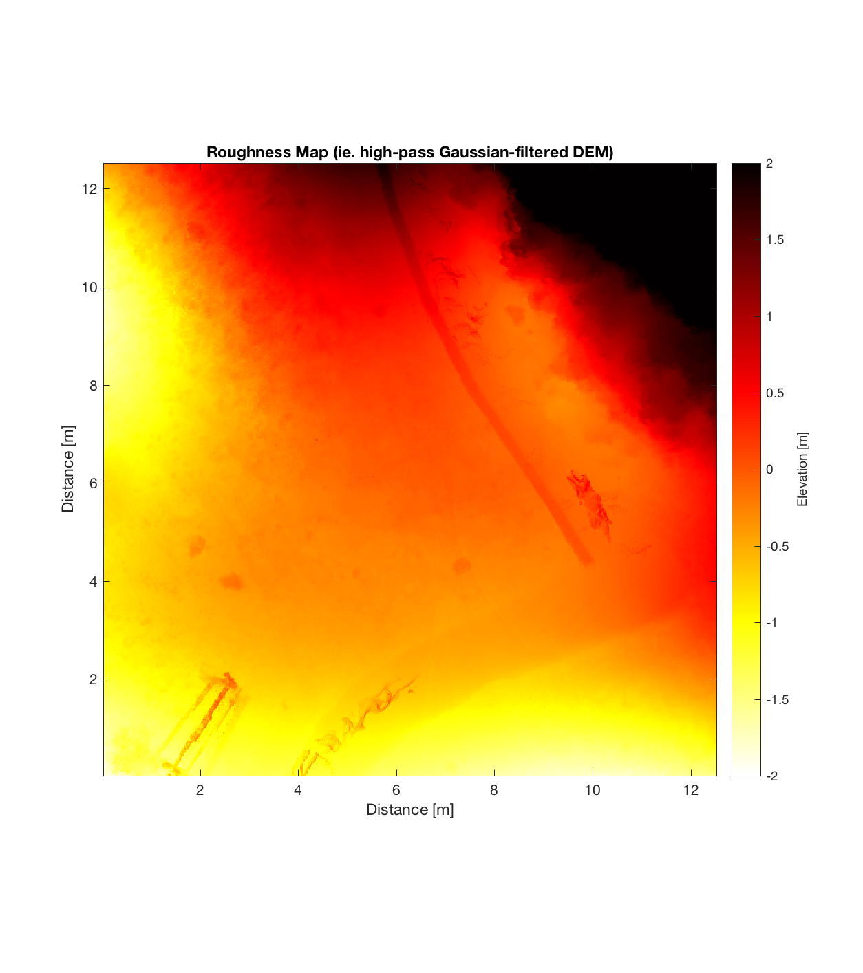
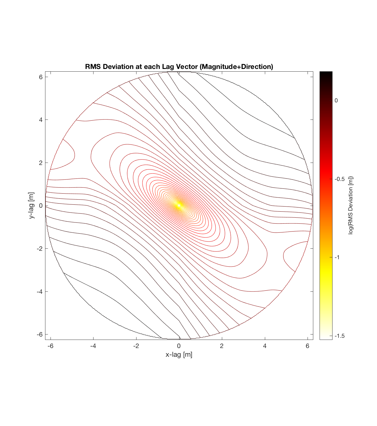
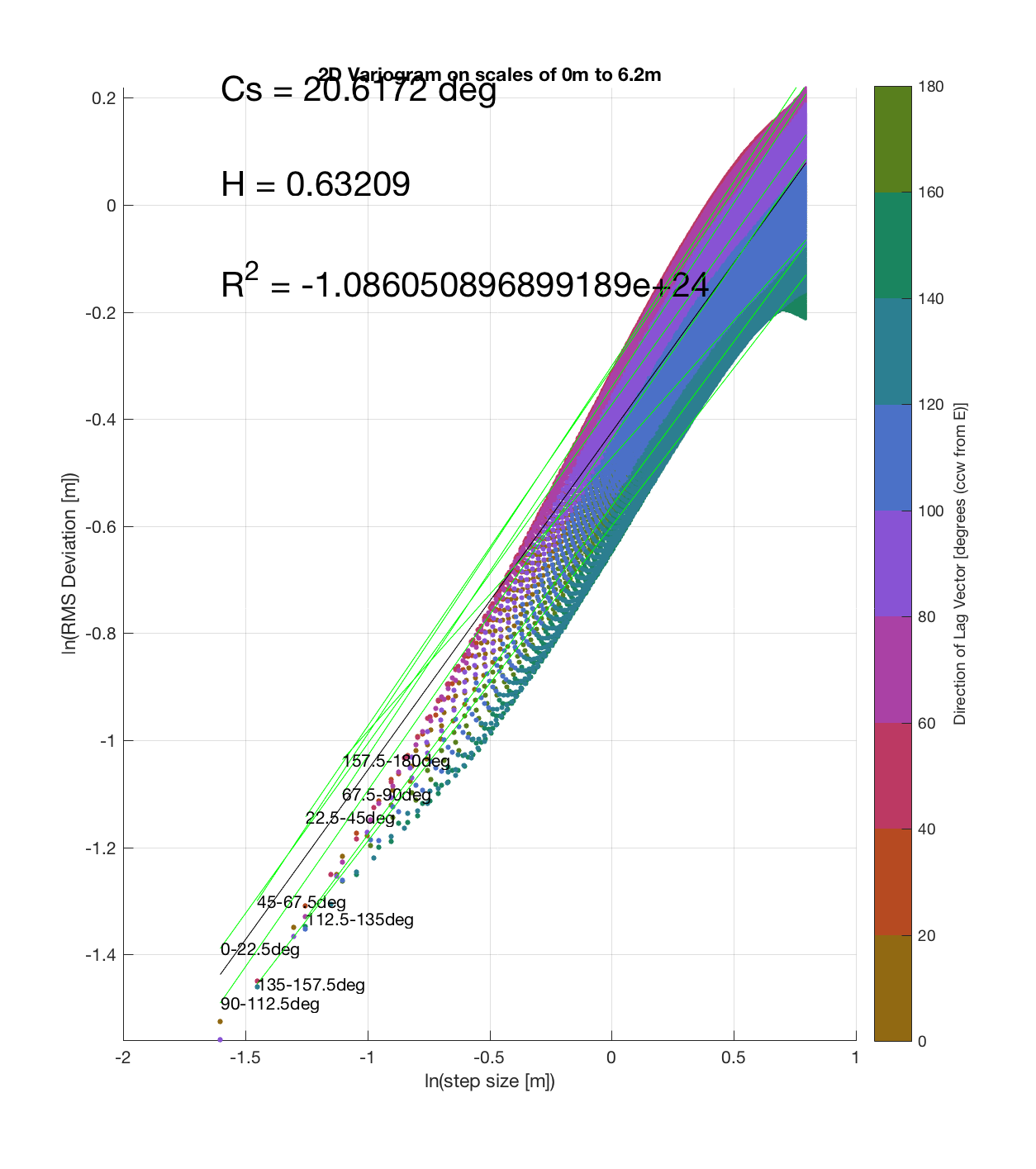
And finally, applying the same procedure at Ina D Caldera:
