China, the World’s Next Reserve Currency: Is De-Dollarization an Upcoming Reality?

By Nuria Bahr and Kavya Vohra

Link to Infographic!

Objectives

BRICS, an intergovernmental organization comprising Brazil, Russia, India, China, South Africa, Egypt, Iran, Ethiopia, and the UAE, collectively cover about 30% of the land’s surface and 42% of the population. Considered the foremost rivals to the G7 bloc – Canada, France, Germany, Italy, and Japan – due to the implementation of initiatives such as NDB (New Development Bank), BRICS Pay, and the BRICS Contingent Reserve Arrangement, the geopolitical bloc in question is arguably growing to place itself center-stage in terms of the global economy. With this in mind, our project intends to elucidate the growing significance of BRICS countries, specifically noting China’s growing leadership within the organization and on the forefront of the global economy.

In order to illustrate exactly how this geopolitical bloc poses a risk to the economic standing of the G7 countries, our project, with the help of data visualization, will also delve into the concept of “de-dollarization” – which denotes “a significant reduction in the use of dollars in world trade and financial transactions, decreasing national, institutional, and corporate demand for the greenback. This would diminish the dominance of the dollar-denominated global capital market, in which borrowers and lenders around the world transact in dollars” (Wise, 2023). Looking at whether de-dollarization is becoming more of a realistic possibility, our project will look into an analysis of “grand debt cycles” that show a repeating pattern of the rise and fall of leading world economies (Monfort, 2024).

Our intended audience would be anybody with an interest in the changing landscape of the economy – but specifically members of the countries that comprise BRICS. We aim to present our project on a website, accompanied by visualizations. Our intention is to put forth our findings in a narrative manner so as to easily convey where BRICS countries stand on a global stage with an emphasis on GDP, import/export of goods, inflation rates, and other statistics that elucidate their growing economic importance.

Data Used

Given that the topic in question surrounded statistics related to the leading global economies in the world, we had a plethora of resources to gather information from. In order to provide the clearest, most accurate narrative, the majority of our dataset was sourced from the International Monetary Fund website (IMF). We used this website to group countries based on geopolitical blocs, grouping BRICS countries together versus G7 countries. We then downloaded datasets for various telling aspects of each group – namely population, inflation rates, GDP, and imports and exports.

Once we had all the required data in Excel sheets, we proceeded to manually clean up the rows and columns to make the data easily digestible for Tableau. This involved removing rows that included headings (to be added back in later) and taking out columns that were descriptive of the type of data being presented, such as “in %”.

Tools Used

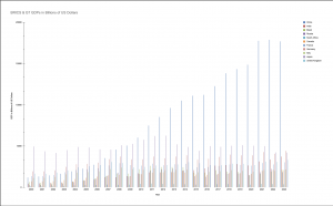
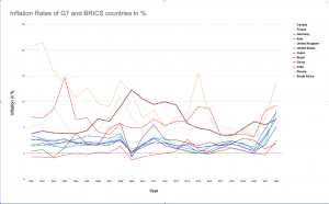
For the initial two graphs which intended to compare GDP and inflation of the BRICS vs G7 countries, we used google sheets, seeing as this was a simplistic visualization. We found this would be the clearest way to aggregate and clean the data, and subsequently produce final graphs on the same platform.

Strengths –

(i) Google sheets allowed us to clean data, view it and produce visualizations all on the same platform. Furthermore, the process of cleaning data, although tedious, was quite simple.

(ii) Easily accessible for simultaneous use, this platform allowed us to work together on visualizations, therefore letting us actively collaborate on creating these visualizations

Cons –

(i) Given that this is a platform designed to bring about fairly simplistic data visualizations, we found it difficult to separate G7 countries from BRICS ones, as sheets didn’t allow us to create seperate groups for each geopolitical bloc.

(ii) We also noticed an inability of the platform to work with larger datasets. Although the data sets we used for these initial graphs were on the smaller, more manageable side – during our preliminary research we found putting larger data sets into the same platform caused lags and crashes on more than one occasion.

After we researched our topic further, and decided to focus more on China’s role within BRICS as compared to our initial plan to focus on all of BRICS, we did not end up using the following graphs in our final infographic:
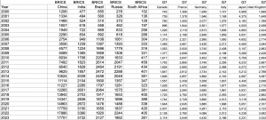
Improved Designs

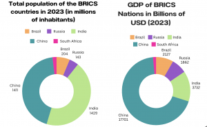
Once we had finalized our nuanced topic we found it best to explore specific aspects of BRICS countries that highlighted where they stood in the global economy. Focusing on GDP, import/export rates, Gross Trade flows and population we created our final graphs.

For population, GDP and import/export rates we used the same method of importing data into google sheets to be cleaned. Following this we created our visualizations on Canva.

Strengths –

(i) Canva’s easy-to-use drag and drop interface has always been a major strength. For these visualizations in particular, once the data was cleaned, Canva was an extremely user-friendly platform when creating the graphs.

(ii) It was important for us to include interactivity in our graphs and Canva allowed us to do this with ease.

Cons –

(i) We noticed that Canva did not automatically code data as expressively and effectively as possible, so this was a manual task that we undertook.
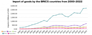
 

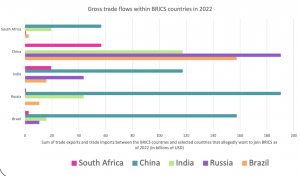
For our 2D graph explaining Gross Trade Flows we found it easiest to import the data into Excel and create a line graph on the same platform.
Analytic Steps

Initially, our project’s aim was to be to portray the BRICS geopolitical bloc as one of growing importance, in every aspect, and furthermore as a true contender for the G7 bloc. As we research data on the members of BRICS, we decided to change our topic to make it slightly more nuanced, as the data we were making visualizations out of, told a more compelling story.

We noticed, especially once we looked at import/export statistics, that China led its allied countries by a vast majority. For example, since 2000, China has consistently been the largest exporter of goods among the BRICS countries, and its share of exports from the bloc has increased significantly. In the year 2000, China’s share of BRICS exports was just over 50%; in 2020, this share has risen to 74%.

Next we looked at Gross Trade Flows, for which we found, now less surprisingly, that China takes up the majority of overall trade within BRICS. With this in mind, our narrative shifted to highlighting the role of China as a leader in the BRICS bloc, as well as a possible contender for the next World Reserve Currency.

Design Process

The first step in the design process was to thoroughly understand the data, including its structure, relationships, and key insights. To this end, we determined the main messages or insights that the visualization should convey. For instance, in the case of BRICS import and export data, the message pertained to trends in trade balances and the relative importance of trade partners, as well as the sheer volume of China’s activities compared to other BRICS nations. Next, we selected appropriate visual encodings (such as line graphs with markers and bar charts) based on the data characteristics and the messages to be conveyed. For line graphs showing trade flows, the choice of lines, markers, and colors helps differentiate between BRICS countries and other selected countries. We ensured that the visualizations effectively communicate the key insights without overwhelming the audience with unnecessary details. This involves striking a balance between expressiveness and effectiveness. The visualizations provide valuable insights to the audience. For instance, the BRICS import and export line graph clearly depicts trade trends over time, highlighting China’s growth and prominence within the space. In terms of soundness, we ensured that the visualizations accurately represent the underlying data without distorting or misleading the audience. This involved careful data processing and understanding. Color coding was used both to differentiate between individual BRICS countries in some cases and to group them against G7 countries as well. This aids in easy identification and comparison between BRICS nations as well as with the wider selected countries depending on the visualization.

The Story

The designed information visualization and infographic offer a comprehensive narrative on the trade dynamics within the BRICS countries and their interactions with other selected nations. Through visually engaging line graphs and comparisons, the visualization highlights the import-export trends of BRICS nations over time, shedding light on key fluctuations and growth patterns. Additionally, the comparative analysis of gross trade flows provides valuable insights into the relative trade importance of BRICS countries within the global context, revealing potential opportunities for economic cooperation and growth. By delving into analytical insights, the visualization identifies emerging trends, challenges, and implications for regional and global economic stability. Ultimately, the narrative concludes with a forward-looking outlook, emphasizing opportunities for collaboration, innovation, and sustainable economic development within the BRICS framework.

Evaluation of Design

Pros:

  • The visualizations provide a clear and concise representation of the data, making it easier for viewers to grasp complex trade patterns and trends. This aids in storytelling by presenting information in a visually intuitive manner.
  • The use of line graphs with markers allows for easy comparison between different countries’ import and export trends over time. Similarly, the separate 2D line graph facilitates comparisons of gross trade flows between BRICS countries and other selected countries, enabling analytical insights into trade dynamics.
  • Visually appealing designs enhance viewer engagement and interest in the data, therefore increasing the likelihood of information retention. This is advantageous for storytelling, as engaged viewers are more likely to internalize the key insights conveyed.

Cons:

  • Some visualizations may oversimplify complex datasets, potentially leading to the loss of nuanced insights. In some cases, the visual representations may not capture all the details or exceptions present in the original datasets.
  • Visualizations may lack the contextual information necessary for a comprehensive understanding of the data. Without additional context or annotations, viewers may struggle to interpret the visualizations accurately, hindering their ability to derive meaningful insights.
  • Certain visualizations, particularly those with complex layouts or interactive elements, may pose accessibility challenges for users with disabilities.

References

Monfort, J. (n.d.). BRICS is intent on de-dollarization but its chances of success are Slim. FXStreet. https://www.fxstreet.com/analysis/brics-is-intent-on-de-dollarization-but-its-chances-of-success-are-slim-202404091602

Munzner, T. (2014). Visualization Analysis and Design (1st ed.). A K Peters/CRC Press. https://doi-org.ezproxy.library.ubc.ca/10.1201/b17511
PMorgan Chase & Co. (n.d.). De-Dollarization. Retrieved from https://www.jpmorgan.com/insights/global-research/currencies/de-dollarization

Ware, C. (2008). Color. Visual Thinking, 65–85. https://doi.org/10.1016/b978-0-12-370896-0.00004-4

Art and Graffiti in Vancouver

Art and Graffiti in Vancouver

By Kelly Chim, Ece Kucukcolak, Riley Job

Wix: https://tabbypublic419.wixsite.com/info419artinvan

Objectives

Vancouver is a city that embraces and encourages art of all forms, but it also emphasises the maintenance of a “clean and natural” city. Thus, what about the more problematic, less recognised and formal artistic mediums? Graffiti.

Where does graffiti lie in the realm of public art?

The legal line between them is defined in the Vancouver bylaws; the two main factors distinguishing it from public art is permission and the property it is on (City Of Vancouver, n.d.). In the past few years, there has been an effort from local graffiti artists to remedy the vandalism problem by advocating for sanctioned graffiti zones (Diment, 2022). In addition, property owners have been open to graffiti murals being painted on their walls as a method of deterring taggers. However, is graffiti culture evolving into a recognised art form, or is it merely a part of city gentrification? Sabina Andron, an expert in urban visual culture, proposes that graffiti are cultural markers that encompass “an urban discourse about plurality and participation, about public space as commons instead of regulated visual space” (2023). Graffiti has value in more than just a nuisance but further in community members trying to establish their vision for their physical spaces.

Our goal is to analyse the locations (neighbourhoods) in which past and present  graffiti and public art are most prevalent, in an attempt to reveal any patterns or trends that may exist, such as whether certain neighbourhoods have a high percentage of both or if the two do not consistently co-exist in the same areas. Our intended audience is Vancouverites who are concerned with community aesthetics and art. What we want to do with these visualizations is collate this discourse into a format that is easily accessible and can be understood by a wide audience to facilitate an important discussion about communal spaces. We want to tell the story about the interaction of formal and non-formal art forms and the way that they interact in Vancouver, a city known for art.


Data Set(s) Used

We downloaded the graffiti and public art data sets from Vancouver’s Open Data Portal and cleaned it. We also downloaded the local area boundary data set from the same site. As we currently live in Vancouver, we wanted to choose data that was relevant to our local area as a way to gain a deeper understanding of our community.


Tools Used

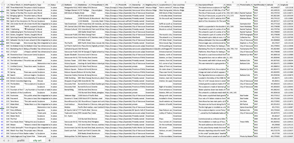
We uploaded our data onto a shared Google Sheets, which allowed us to work from and clean the data together to ensure that it was thorough. We matched neighbourhood names across both data sets, as well as filled in cells that were missing information, such as location coordinates. To accomplish this, we relied on Google Maps to visually search for the art and then copied the coordinates onto Sheets. This was helpful in finding most of them, but did not work specifically for art that also served as public infrastructure such as painted benches, engraved manhole covers or advertisements and posters that had multiple undisclosed locations. Thus, we deleted several cells where the artwork’s locations were difficult to pinpoint or scattered across a stretch of land as there was no proper documentation about their locations. We also realised later that to upload custom coordinates in Tableau, latitude and longitude had to have their own columns, so we separated them accordingly as the datasets had them combined into one column. When we were finished, we exported the Sheets as an Excel file. We decided to keep the Graffiti and City Art data sets separate as the Graffiti sheet had substantially fewer different types of information than the city art sheet.

Fig 1. Graffiti Data Set (Excel)

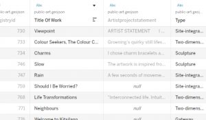
Fig 2. City Art Data Set (Excel)

Following this, we brainstormed a couple of ideas for the visualisations.


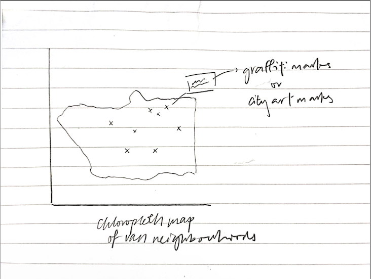
Fig 3. Brainstorming Sketch

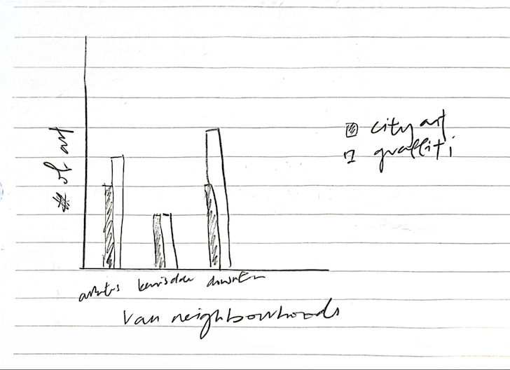
Fig 4. Brainstorming Sketch 2

After this, we ingested the data in Tableau. We used the software to assign our custom coordinate fields with “latitude” and “longitude” geographic roles to help plot these points on the map. To create our visualisations on Tableau, we referred to previous class exercises, online videos, discussion forums, and also had the professor’s help to guide us in the process of visualising our ideas. It was especially useful in helping assign the right attributes across multiple data sets, as well as helping us layer maps to show different attributes. Tableau, despite being a more difficult software, was suitable for our project because of the skills we had learned in class already and was useful in visualising large amounts of data.

We then used Wix to create our story for the final submission. It allows us to include embeds of Tableau graphs, and also has many graphics and text options for us to create an engaging story on a platform that’s relatively easy to navigate.


Analytic Steps

From our research about the graffiti art scene we determined that the existing view on Graffiti in Vancouver is mixed due to inconsistent municipal funding, public dislike of tagging but positive towards legal communal murals and had a successful community group, the Vancouver Coalition of Graffiti Writers, before its shut down in response to mayor Ken Sim’s new anti-graffiti policies in 2022 (Kozelj, 2022; Robinson, 2021). As there are such wide ranges of opinion and legality surrounding the graffiti scene we wanted to tell a story that invokes critical thinking from the audience, rather than in a persuasive narrative format.

We were pretty certain of the idea we wanted to communicate from the start, as seen in the Figure 3 sketch, but were unsure of the type of graphs we would discover as a result of our data. As out topic considers the geo-spatial location of graffiti and city art we wanted to ensure that locational data was the focus throughout our slides and visualizations. We conducted a few visual explorations of the geographical data to determine which graphs convey information in an aesthetic and clean way.

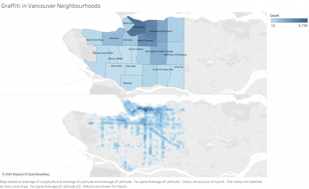
Figure 5 below shows one of our first drafts where we split the graph into two; both illustrated the number of graffiti in each neighbourhood (as shaded regions and as a density map). We followed effectiveness in choosing to utilize luminance to codify region as position, length, tilt and area were already being utilized to define different neighbourhood boundaries and land formations in the above visualization (Munzner, 2015). However, as spatial position is so expressive we wanted to ensure that it was being utilized in the density map to show exactly where the incidents occurred by using circular marks. The use of luminance in showing density also is a great avenue for this visualization due to humans’ increased sensitivity to spatially arranged data when encoded by luminance (Ware, 2008). However, we decided to improve on this visualization by combining them into one unified map later on for a clearer comparison.

Fig 5. Draft of Graffiti in Vancouver Neighbourhoods (Tableau)

Figure 6 below is another one of our drafts where we used a labelled, stacked bar graph to demonstrate the contrast between the number of graffiti versus the number of city art in each local neighbourhood. However, we found that it was not useful to compare the relative compositions of art in each neighbourhood because the varying heights complicated the comparison between the two categories. Thus, we decided to move away from the stacked bar chart method and instead used a grouped bar chart as seen in Figure 9.

Fig 6. Draft of Graffiti VS City Art in Vancouver Neighbourhoods (Tableau)


Design Process 

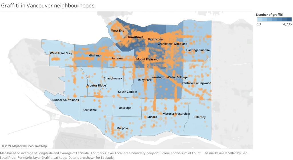
Basing the graffiti map on Figures 3 and 5, we first worked on layering the data sets with a choropleth map and symbol map for graffiti found in local neighbourhoods: both deal with graffiti in different ways, the choropleth map makes use of luminance (saturation) to visualise each neighbourhood’s graffiti count while the symbol map overlays the exact graffiti locations onto the map with circular marks (Figure 7). As such, no other data type was introduced in this visualisation, following the expressiveness principle. To contrast against the blue stepped colours of the choropleth map, an orange hue was used for the symbol map, increasing the marks’ saliency. Thus, the most important attribute of graffiti location was expressed through position and hue, following the effectiveness principle.

Fig 7. Graffiti in Vancouver Neighbourhoods (Tableau)

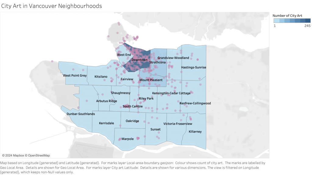
We repeated the method used to create the graffiti map for the city art one, but also included more details about the art as well that can be viewed if hovered over (Figure 8). These interactive elements were included as we thought it would be helpful to include pictures and descriptions of the artwork, but did not want to overcrowd the visualization with (unnecessary) information, thus, following the expressiveness principle. In terms of the hue choice for these maps, although we kept the same blue stepped gradient for the chloropleth map as in Figure 7, we decided to choose a lighter, less-contrasting purple hue for the city art marks. This is because we wanted to juxtapose the city art map with the graffiti map. Additionally, as orange and blue are complementary colours, whereas purple and blue are analogous, it plays into the metaphor that people believe city art (purple) belongs in the city while graffiti (orange) does not. Hence, although we did not strictly maintain effectiveness with hues in this visualisation, it still comes across with the geographical positions of the city art.

Fig 8. City Art in Vancouver Neighbourhoods (Tableau)

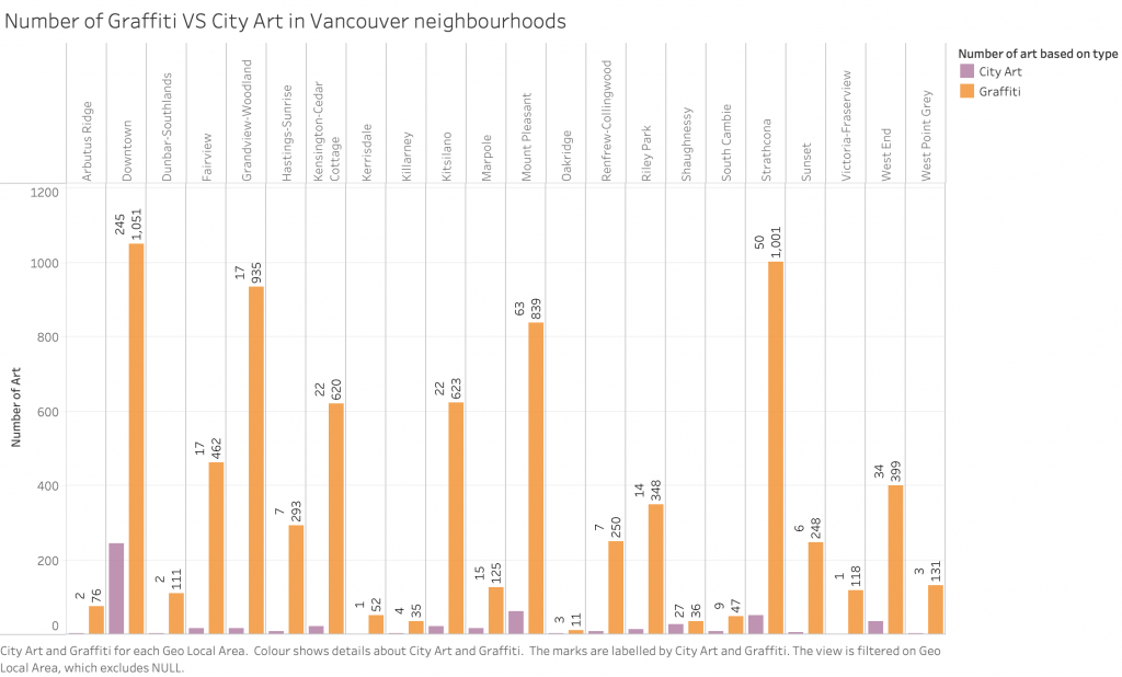
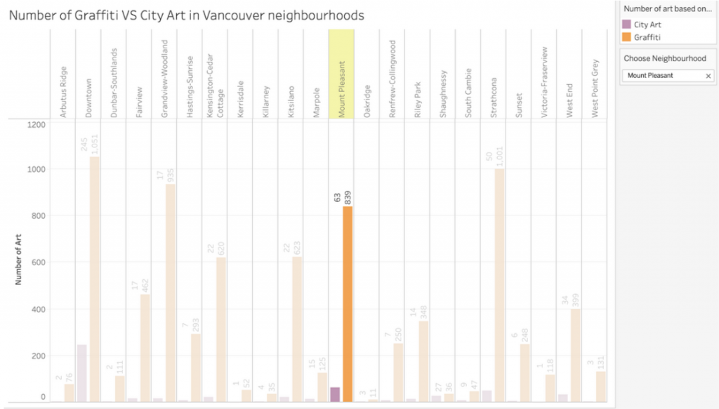
The visualisation in Figure 9 is a grouped bar chart that compares the graffiti count and the city art count for each neighbourhood in a simple manner, as well as makes use of an interactive highlight feature (seen in Fig 10) to allow users to spotlight or find a specific neighbourhood quickly and easily. To be consistent, we chose to use the same colours for the “graffiti” and “city art” measures as they were used previously in Figures 7 and 8. Additionally, the visualisation uses an identity channel and is organised alphabetically by neighbourhood, following the expressiveness principle.


Fig 9. Number of Graffiti VS City Art in Vancouver Neighbourhoods (Tableau)

Fig 10. Interactive Element: Number of Graffiti VS City Art in Vancouver Neighbourhoods (Tableau)

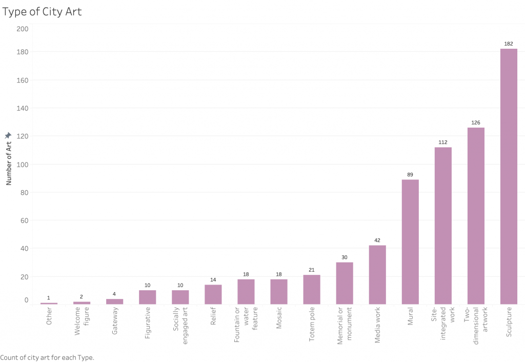
Figure 11 looks at a different visualisation altogether, focusing on the type of city art that exists within Vancouver. We decided to arrange it by increasing values for the number of art per city art type rather than alphabetical order because we believe the focus should be on which city art type is most prevalent, thereby following the effectiveness principle. The expressiveness principle is also taken into account as only the relevant information is shown in the visualisation, keeping the graph clean and easily understood by viewers.
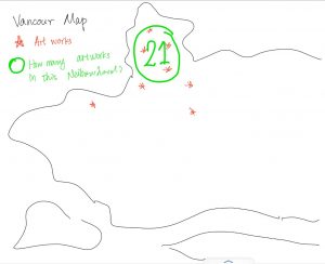
Fig 11. Types of City Art in Vancouver (Tableau)


The Story

After finishing the visualizations, we planned to use Canva for our presentation. However, we discovered that Canva did not support embedding our graphs, so we switched to Wix. Wix allowed us to embed the visualizations and include interactive elements.

Our project focused on analyzing the dynamics of graffiti and public art within Vancouver’s urban landscape. We identified areas where these art forms are most common; in some neighborhoods, there is more of a coexistence, and in others, a scarcity. We wanted to create a discussion on public spaces and the transformation of graffiti from vandalism to a recognized art form. We examine how it either integrates with or conflicts with the city’s design.


Pros and Cons

Pros: We used geographical maps and bar graphs to help us present the distribution and volume of graffiti and public art across Vancouver in an easily understandable way. This approach makes the data accessible and interpretable to a broad audience, which creates a compelling visual story.

Furthermore, we incorporated interactive elements like hover-over details in Tableau to improve the user experience. This feature allows the users to engage and explore specific artworks or graffiti which gives them more context. Displaying graffiti and public art data side by side, we created a comparative analysis. This helps to show the audience the frequency and acceptance of these art forms in different neighbourhood’s.

Cons: Our analysis is limited by the available data sets, therefore it may not fully capture the amount and exact location of graffiti and public art. This limitation could lead to potential biases or gaps in our analysis which can affect the overall narrative and conclusions that we came up with. The design choices and story structure in our project could impact  audience opinion and influence whether graffiti is viewed more positively or negatively. This could affect the objectivity of our analysis and the message we intend to convey. We tried  to make our project as accessible as possible, there’s a risk of oversimplifying the complicated relationship between graffiti, public art, and Vancouver’s landscape. This could mean overlooking deeper narratives and biases.


Bibliography

Andron, S. (2024). Urban surfaces, graffiti, and the right to the city. Routledge.

Andron, S. (2023). Urban Surfaces, Graffiti, and the Right to the City (1st ed.). Routledge. https://doi.org/10.4324/9781003456070

CBC/Radio Canada. (2017, February 24). POV | 21 of my friends died from fentanyl overdoses, now I paint murals to stop others | CBC Radio. CBCnews. https://www.cbc.ca/radio/nowornever/how-to-unleash-your-inner-artist-1.3995740/pov-21-of-my-friends-died-from-fentanyl-overdoses-now-i-paint-murals-to-stop-others-1.3997737
City Of Vancouver. (n.d.). Graffiti By-law 7343. Vancouver. https://vancouver.ca/your-government/graffiti-bylaw.aspx

Diment, M. (2022). Vancouver now has its first legal ‘graffiti wall’ and more could be in the works. Vancouver is Awesome. https://www.vancouverisawesome.com/local-news/first-legal-graffiti-wall-alley-tagging-vancouver-bc-5707660#google_vignette

Kozelj, J. (2022). Vancouver’s So Nice. Where’s the Graffiti?. The Tyee. https://thetyee.ca/News/2022/11/22/Vancouver-So-Nice-Where-Graffiti/

​​Kulkarni, A. (2024, January 15). Vancouver art students to learn about graffiti from one of the city’s Masters | CBC News. CBCnews. https://www.cbc.ca/news/canada/british-columbia/smokey-d-art-class-1.7083674

Robinson, K. (2021). Vancouver sees 70% spike in nuisance graffiti reports to 311 during COVID-19 pandemic. Global News. https://globalnews.ca/news/8240692/vancouver-spike-nuisance-graffiti-calls-311-covid-19-pandemic/

Smith, S. (2014). Forty Years of the Cadillac Ranch. Texas Monthly. https://www.texasmonthly.com/travel/forty-years-of-the-cadillac-ranch/

Images 

Top-Calligrapher-266. (2022). Vancouver, BC – Graffiti.

https://www.reddit.com/r/Graffiti/comments/w65h34/vancouver_bc_graffiti/

Walker, J. (2010). vancouver: the almost perfect grid. https://humantransit.org/2010/02/vancouver-the-almost-perfect-grid.html

Spotify Stats 2023

By Lakshanyaa Ganesh and Aarthi Krishnan Sharma

Tableau Links:

Dashboard 1 (click for interaction):

Dashboard 1


Dashboard 2 (click for interaction):

Dashboard 2


Canva Infographic (volume up!):

Background and objectives

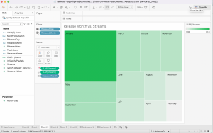
Presently, Spotify publishes listening statistics for the past year through Spotify Wrapped at the end of every year. It presents data of the individual user, covering parameters such as Top Artist, Top Genre, and Top Song to name a few. It also does the Artist Wrapped, which tells artists how much their music has been listened to. The parameters that we discovered in this data set were unique and more niche, such as the number of playlists the song was added to on Spotify, Apple Music, Shazam, and Weezer, as well as the number of times it charted on each of those platforms. We wanted to focus our analysis on Spotify and examine the correlation between the total number of streams of a song and the number of playlists it has been added to, and also if the month and/or day that songs are released play any role in how popular they become. 

We wanted to support the production of new knowledge and communicate these trends through the data as it presently stands. Since this data is not readily available to the public, we hope that our current visualizations will be interesting and engaging for our audience of Spotify users who are very interested in and engage with Spotify Wrapped to learn more about the listening patterns of the world. According to the levels of interaction as described by Heer in “Interactive Dynamics for Visual Analysis”, we are hoping that those interacting with our visualizations can participate in high level interaction, where they discover trends and connections between data through our Tableau dashboard, and also are presented the information in an eye-catching, enjoyable way through our static Canva infographic (2012, p. 2).

Details of the dataset

We used the dataset “Most Streamed Spotify Songs [in] 2023, which we found on the open source data website “Kaggle”. It is most likely derived from Spotify API (Spotify’s platform for developers), thoughit was difficult to find the exact source of the data. This kind of data, especially the more niche parameters available through the dataset, is not readily available in the public realm, It can therefore be relatively safe to assume that the data has been extracted from Spotify by the publisher. The data also has a usability score of 10 out of 10 on Kaggle. This additionally includes scores on its completeness, credibility and compatibility. We also found that the publisher of the dataset is a data scientist who has published many other reliable datasets on Kaggle. These factors confirmed the validity of the data to use for our visualizations.

The file has 943 unique entries, with 24 parameters. Apart from the attributes “track_name”, “artist(s)_name”, “key”, and “mode”, all of which are strings, the rest of the attributes are integers. We were able to manually clean the few instances of wrongly formatted data and also were able to run it through Tableau Prep to confirm that the dataset as a whole is valid. Out of all the available attributes, we only used a few: track_name, artist(s)_name, “released_year”, “released_month”, “released_day”, “in_spotify_playlists”, and “streams”. For the sake of this project, we decided to use the top 250 entries by streams.

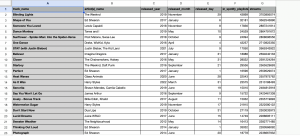
A snapshot of our cleaned data

In terms of the data itself, we found that a key weakness was in the fact that the data was cumulative. Since the data shows how many streams and how many playlists a certain song has accumulated since its release, it makes sense that songs released prior to 2023 have more streams. It would have been more beneficial and more fair of a visualization if streams were counted per year.

Tools: strengths and weaknesses

Tableau proved to be a very useful tool in exploring this dataset. Due to the size of the dataset, Tableau proved to be useful in allowing us to adjust and modify the parameters, as well as view and analyze individual data points in the views that we created. The brushing and linking feature in particular helped us in creating effective interactive dashboards. As we are relatively new to using Tableau, this was slightly difficult to implement at the beginning, where we did not include our switch as one of the parameters in Dashboard 2, so the sheets were not linked as we wanted. We were eventually able to achieve the effect that we wanted, but it took a lot of trial and error within the software. A shortcoming of Tableau in this sense is that it is a very complex software that is not always easy to manipulate in the exact ways that we want on the first try. However, there are not many other softwares that would allow us to deal with a dataset of this size as effectively as Tableau would.

In comparison, Canva was a lot easier to use, as both of us already had experience using it for various other purposes. It is a graphic design software that is extremely user friendly, allowing us to manipulate objects and their positions very easily. We also had a rough idea of the kind of visuals we wanted to use based on Spotify Wrapped, so we were able to implement those in a relatively straightforward manner. Since the task we had to do with Canva (summarizing findings from our dataset and dashboards) was simpler than what we had to do with Tableau, we did not run into any major issues with using this software.

Understanding our data

At the beginning of our project, we had a very good idea of what our goals with our project were, and we knew which parts of the dataset we wanted to analyze and use specifically: the track names, artists, release dates, the amount of playlists they were in, and their total streams by the end of 2023. We had a general sense of wanting to see if there were any differences between song streams versus how many playlists they were in, and if release dates had any significance or correlation to streams at all. 

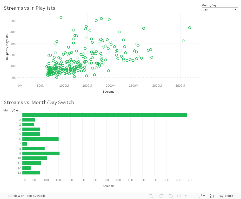
We were not able to solidify any specific patterns, however, until after we began to focus on creating visualizations to communicate the data effectively. Over the course of the project, we were more focused on communicating existing data and analyzing its trends visually as opposed to producing anything new from insights derived just by reading the dataset itself. When we began creating visualizations, we began to notice significant trends in how January seemed to be a very successful month for songs to be released, as well as the first of every month. We also found that the popularity of songs seemed to differ when comparing streams versus the amount of playlists certain songs are in – some songs might have a low number of streams but are in many playlists or vice versa. 

Design process

Although we did not start our project by creating sketches, we were eager to explore Tableau, so we spent time doing trial and error with it, creating multiple different views to see what would best represent our data, and used the most relevant ones in our dashboard. We did also keep the ones we did not use in the dashboards, for us to keep track of our design process. We had a rough idea of the interactions that we wanted to create, such as linking the months and days to the individual data points of each song (Dashboard 2). Even though we did struggle with it initially, we were able to implement the brushing and linking using prior knowledge gained through the class activities and assignments. 

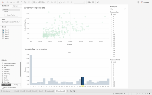
An early version of one of our dashboards

A view that we created and like but ultimately did not use

We also believe that our visualization was expressive and effective, as we attempted to match the attributes to the right kinds of data, and as a result, the most salient channels according to their importance in our visualization. According to Munzner’s ranking (Munzner, 2015), our data was encoded using the following channels:

  • Month (ordinal data): Length – 1st on Munzner’s ranking
  • Day, Released Year, Streams, In Spotify Playlists (quantitative data): Position – 2nd on Munzner’s ranking
  • Artist Name, Song Name (categorical data): viewable through interaction of hovering

In terms of maximizing the expressiveness of our data, we picked the most important data to communicate visually: the dates of song release as well as popularity in terms of streams and number of playlists. Since all of this data is quantitative in nature, we primarily used the magnitude channel to encode all of this information. To maximize expressiveness, our visualizations still show all of the data such as track name and title when the user hovers on all of the data points, but since these attributes are categorical and there were 250 individual data points, we did not want to crowd our visualizations through expressing each individual artist and song name. 

The Story

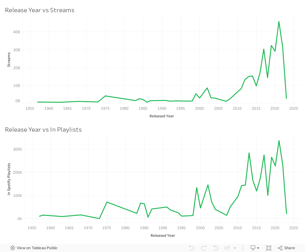
Through our InfoVis and Infographic, we want to tell the story of the most popular songs and artists on Spotify, as well as the most popular release dates (months and days) that get the most amount of streams. We also wanted to add the extra dimension of the amount of playlists songs are placed in, and if this says anything about a song’s popularity. We found that 2021 was a good year for music, with the most streams peaking that year along with the number of playlists songs from that year were saved to. As this dataset is cumulative, there are more streams for the songs that were released in earlier years as opposed to in 2023. We also found that streams do not necessarily dictate popularity, as the songs that came out in 2013, 2017, 2019, and 2021 were in the most amount of playlists. 

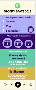
It was also interesting to look at 2013 in particular. The number of streams in total for that year was not that high, but the number of playlists that songs from 2013 were saved to peaked. According to a Billboard article by Andrew Unterberger, the rise in popularity of streaming through YouTube music and other online platforms helped streaming platforms like Spotify to explode in use. This can be one of the reasons why songs from that year that were newly released garner more streams and gain popularity. We also found that songs released in January had the most number of streams, whereas songs released in February had the least. We also found that songs released on the first of every month had the most number of streams by a landslide, whereas songs released on the 7th had the least. The 21st and the 9th of the month were also successful release days for streams. 

There are outliers to these trends, however. Blinding Lights by the Weeknd came out on November 29th (both an unpopular day and month for a song to be released) but still had the most streams and was in the most amount of playlists. Shape of You by Ed Sheeran was also an outlier song. It came out on January 6th – whilst January is a successful month for streams, the 6th is not a popular date. On the other hand, Get Lucky by Daft Punk and Wake Me Up by Avicii both came out on January 1st but did not receive many streams. Get Lucky is saved to many playlists, however, in an inversely positive relationship with the number of streams it has. The popularity of songs released in January may be due to market concerns, given that the market is significantly less saturated at this time, according to a Bandsintown article by Randi Zimmerman. They also state that January is also when people tend to be more likely to branch out in general and try new things, which applies to new music as well. 

Pros and cons of our design

We feel that we have curated our views in a manner that is conducive to telling the story that we just described. The individual outliers that we mentioned are easily visible in Dashboard 2, as they are clearly distanced from the larger cluster of data points. More information about each data point, such as the track name, exact number of streams and number of playlists it is in, as well as the year, month and day it was released. The availability of this additional information allowed us to craft a more well-rounded story, which does not just point out trends and outliers, but allows the audience to view the additional factors which may have contributed to a song’s position on the dashboard. Data points like Get Lucky and September proved our hypothesis that the number of playlists a song is in is an adequate measure of its popularity, whereas songs like Someone You Loved and STAY disproved this. A main con of this dashboard was that there were 250 individual data points fit into the Streams vs. In Playlists view, which made it slightly messy to look at. However, the fact that we brushed and linked it to the Streams vs. Month/Day switch made it easier to identify trends, as clicking on the bars in this view highlighted the corresponding data points in the Streams vs. In Playlists view. 

The first iteration of our infographic – too much information, too little space

Due to the fact that the data was a bit crowded on Tableau, we created the additional visual on Canva to consolidate our information and point out the important facts from our story. We started off by creating a traditional infographic, but realised soon into the process that this was not entirely conducive to the amount and kind of information we wanted to convey, as it was too cluttered and crowded. As a result, we decided to pivot to a slide format, in order to break down the information into smaller sections, for improved effectiveness and digestibility. We created this to present our story in a more visually appealing and attractive manner that we were not able to do with Tableau. Using the colour drop tool, we also used the exact hues from Spotify Wrapped 2023 to make our story look more cohesive and in line with the Spotify brand. Additionally, since we chose not to represent textual details of our data points overtly in Tableau, we chose to collate and present them here.

References

Aswad, J. (2020, July 5). The Weeknd Talks ‘American Dad,’ and What Most People Don’t Know About Him. Variety. https://variety.com/2020/music/news/the-weeknd-american-dad-what-people-dont-know-1234695111/

Capaldi. (n.d.). Lewis Capaldi. YouTube Music. https://music.youtube.com/channel/UCxrxwFTBU3DTJ9Y5TKeW7KA 

 Cole, R. (2024, April 7). Ed Sheeran | Biography, Songs, Wife, & Facts. Encyclopedia Britannica. https://www.britannica.com/biography/Ed-Sheeran

Elgiriyewithana, N. (2023, August 26). Most streamed Spotify Songs 2023. Kaggle. https://www.kaggle.com/datasets/nelgiriyewithana/top-spotify-songs-2023?resource=download

Heer, J., & Shneiderman, B. (2012). Interactive Dynamics for visual analysis. Communications of the ACM, 55(4), 45–54. https://doi.org/10.1145/2133806.2133821

Munzner, T. (2015). Visualization Analysis and Design. Boca Raton, FL: CRC Press.

Rubin, R. (2021, December 16). The best and worst months to release music. Bandsintown for Artists. https://artists.bandsintown.com/support/blog/the-best-and-worst-months-to-release-music

Unterberger, A. (2020, April 14). 2013 was the year that… streaming officially became Unignorable. Billboard. https://www.billboard.com/music/music-news/2013-year-of-streaming-8545169/

ICBC Crash Report from 2018 to 2022

ICBC Crash Report from 2018 to 2022 


Links to Our Project

Interactive Map link:

Final Police Reported Map: Dashboard 1 – Tableau Cloud

Figma link: https://www.figma.com/proto/9jDv4Hv4gtFASMASFQVs3I/INFO-419-Infographic-Final


Introduction 

Transportation is an essential part of each person’s daily life. You could be driving, walking, busing or biking. But when we are doing these things we never think of the possible accidents that can occur.  We are all at risk when we are out on the roads. The Vancouver Sun has reported that over the past 5 years there have been more that 400,000 car crashes in the lower mainland (Griffiths, 2021). During the years from 2000 to 2019 Statistics Canada reported that the number of registered vehicles in Canada has increased from 17 million to 25.4 million (Government of Canada, Statistics Canada, 2022). Every day there are over 760 crashes in BC (Injury Topic – Road Safety | BCIRPU, n.d.). It is evident that with the increased cars on the roads this is an important topic to analyze and discuss.  By examining the crash reports provided by ICBC we want to reveal the hazard when it comes to being on the roads and come up with potential solutions. This information would also inform the public of what to be aware of when they are on the road. 


Objectives 

The objective of our InfoVis has 2 main goals. The first one is from a high-level action perspective. At this level we want our audience to gain new knowledge from our visual analysis. We want our audience to uncover and be able to comprehend the patterns that they are not able to see in the spreadsheets. We mainly want our audience to discover what areas in the lower mainland have the highest number of car accidents, what weather and road conditions cause the most accidents. By providing this knowledge to the general public about this, it will inform them about the potential risk when they are navigating the roads as well as helping them make a safer choice. The second goal of our InfoVis is at a mid-level action perspective. We want policy makers and the local authorities to look at the visualizations we have made and highlight the importance of it to future drivers. They could implement this into the writing sections of the drivers test.  

Changes

Our work didn’t divert much from our original project plan. Small things came up such as only using the police-reported crashes rather than both police-reported and insurance-reported crashes due to the difficulty in using insurance-reported crash data. At one point we had intended to compare the two data sets to investigate differences in trends, but that idea just wasn’t possible with the datasets, tools, and time we had for this project.

Data Used 

For this project, we used a dataset that was accessed through the DataBC provided by ICBC. This dataset included police-reported crashes from 2018 to 2022. This data is appropriate for our project because ICBC is a credible source and can be referenced. It also operates with the government, and it plays an important role in the insurance industry. They collect a large amount of data in this industry making it reliable and credible. The information that the dataset included collision types, crashes per month and year, crashes in each municipality, what kind of weather the crashes happened in, whether a cyclist and a motorcycle were involved, crash configurations, collision type, if it was a hit and run, if an animal was involved, if a pedestrian was involved, the road conditions, weather, number of casualties, and the total numbers of vehicles involved. We chose to work with their police-reported crashes data rather than all ICBC insurance reported crashes as the dataset was more manageable (smaller in size), cleaner (few to no null values), and had all the data fields we were interested in.

Additionally, we needed to compile a GeoJSON file for the lower mainland of BC spatial data so we could map out the boundaries for our visualization map. While initially we tried using polygon data from the BC government for legal municipality boundaries, not all municipalities written in the police-reports were legal municipalities with clear boundaries. We ended up deriving our own coordinate point data as a CSV spatial file using a mixture of Google maps and latitude.to to identify approximate centers of each area listed as a municipality. While this is an imperfect method of data collection, we went to great lengths to check that each of the map points in google maps, latitude.to, and in Tableau were accurate to the municipality or unincorporated community’s location.


Tools Used 

The main tools that we used to design our InfoVis for our project are Tableau Desktop and Figma. In Tableau Desktop we used it specifically to create our graphs. We used Tableau Desktop to create our graphs since it was user friendly to us because we learned how to use it in class and could reach out to our professor for help if we ever run into any difficulties. The other tool we used was Figma.We used Figma to create and infographic. In our original proposal, we were going to use Canva or WordPress but when using WordPress to create a site I ran into some issues with loading the site so I switched to Figma as I had some experience with it and I have never encountered problems regarding the site loading.

As mentioned in the data section, the Government of BC data Catalogue, Google maps, and latitude.to were used for data collection.

Analytic Steps

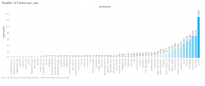
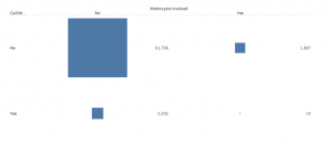
The data we used required a lot of analysis. We had to create many rough visualizations just to understand the data better ourselves, and ultimately needed many visualizations to communicate the data’s story. First, we picked a couple of things that we thought would be interesting to look at. For example, we knew we wanted to look at which areas had the highest amount of car crashes and how weather affects the amount of car crashes. Then we played with the data in Tableau Desktop to see if there was anything that stood out to us. We included graphs that show what municipalities had the most amount of crashes so people would be aware of this. Then we also included a graph by year and month showing how many car crashes. We wanted to include this because the data we used included the year of 2020, which was during the pandemic. We wanted to see if there was a correlation between the number of crashes and the restrictions of COVID-19. Then we included a graph about how many crashes occur during specific weather. We found this graph very interesting as it shows that there are more crashes on clear days as we thought there would be more crashes on rainy weather as there is an increased chance of occurring. We found that there were more cyclists involved in crashes instead of motorcycles, but that the vast majority of crashes were between vehicles.


Design Process 

For the website/infographic we created we first brainstormed a list of interesting correlations in the ICBC data. Then we created a general outline of what we wanted the website to look like.

After we got the basic outline of what we wanted it to look like we then decided on the main colors we were going to use.  We went with the ICBC blue and created a small car logo to match the topic we were talking about.

We then made the visualizations for those data fields while paying attention to the expressiveness and effectiveness of the visualization elements. First we just used the general colors that Tableau Desktop automatically chooses but then we noticed that we should make graphs that have more than one colour, user-friendly to people that are color blind. When using expressiveness and effectiveness in our graph we used color saturation to show which municipalities had the least to most crashes. 

We also used area(2D size) to show the amount of motorcycle vs. cyclist involved.


Once we had all of the graphs that we wanted created, we had to think of the flow of the infographic. First, we decided that starting with a small introduction about the topic would be a good way to lead our audience into what would be informing them. Then we dive into the statistics of our graphs, we begin with the trends of crashes over the five years as this sets a general idea of the numbers for crashes and it sets us up to analyze the possible reasons for these numbers we would be discussing later on. Then we would specifically look at municipalities and the number of crashes they had to give us insight into the graphical variation across the lower mainland. Then we would discuss the weather influences and cyclists’ involvement in the crashes and conclude our findings. 

In addition to the infographic demonstrating key information in the ICBC’s police reported crash data, we also wanted to create a more free-form and exploratory visualization of the data. We created an interactive map that allows people to search, browse, and filter through the data field categories to investigate any specific data items of interest to them. Using the map allows people to look at specific areas of the lower mainland that might affect them personally, and see connections between location, crash counts, and any filters they choose to use. While the infographic used a blue theme for colours, orange was chosen for the map to maximize its popout effect from the grey and white background. Especially because most of the data points are of the lightest shade, the orange colour is much more visible than the light blue.


The Story & Key Findings 

The two visualizations work together to tell the story of where, when, and how car crashes occur in the lower mainland. The interactive map creates a more accessible way of investigating the data for any trends related to location while the infographic breaks down some of the specific findings that are important to take away from the data set. 

First and foremost, Surrey has a significant amount of police-reported crashes compared to any other municipality. Looking in a slightly larger area, most crashes are in the metropolitan area showing us that population dense areas where there are more cars and tighter roads have more crashes. While this might seem obvious at first, the large difference in the quantity of crashes will hopefully encourage people to drive more cautiously in these metropolitan areas, and for policy-makers to see health and safety value in reducing traffic and cars on the road in these areas.

In our infographic we include a chart depicting a comparison between crashes involving cyclists and motorcycles. We can see that the vast majority of crashes are between two vehicles, but also that cyclists are involved in crashes more frequently than motorcycles. While motorcycles will have to be on the same roads as cars, creating cycling infrastructure to separate cyclists from vehicles could have a very significant impact on reducing crashes. Hopefully this visualization will help people be more aware of the dangers of having cyclists on the road, support such infrastructure change policies, and be more aware of cyclists while they are driving. On the other hand, cyclists viewing this visualization will hopefully understand the significant risk they are putting themselves in when they bike on the roads, and will opt for routes that do have dedicated bike lanes, and to be very cautious at all points where cars could hit them.


Pros & Cons

Our visualizations help explore the complicated crash statistics in a more user-friendly, and in a more digestible manner rather than just having to look at an Excel spreadsheet alone. However, one thing that Figma did not allow us to do is embed our map into the site which we did not notice until the very end of completing our project.

Another benefit of having these visualizations is that they are in a much more shareable format than the data sets. By having pictures, figma links, and tableau links, people can share them digitally with ease. The large excel spreadsheets of the ICBC data can be downloaded, but not understood and communicated to people without a fair deal of work. Our visualizations will make the data findings much more accessible, and shareable.

Our visualizations are not perfect. While they do present a certain story and point of view, creating a larger and broader project would provide a lot more relevant context for understanding data points. Car crash numbers can be helpful for understanding the scale of the problem, however measurements of risk, and increases of risk in certain areas would be more accurate for showing the places and conditions that require more caution and policy changes. For example, the data showing weather conditions during these crashes would make more sense within the context of crashes per rainy day, and per clear day. This would require knowing the amount of time during the year it was raining, what time of the day it was raining, and then the time of day for the crashes. With more time, we could’ve gotten a weather conditions data set, analyzed it, and cross-referenced it with the crash statistics to create such an evaluation.

Our map is also limited by the abilities of Tableau interactions. Ideally the map could be more interactive such that zooming in and out of the map would act as a filter for the municipalities included in the column chart, however Tableaus doesn’t have this functionality. Furthermore, With more time we could’ve made a visualization for each data field such that clicking on a filter would add a visualization to the dashboard of crash counts for that data field item. This would increase the interactivity, and the number of conclusions that could be drawn from the map.

Conclusion

This project is fairly to the point. We took ICBC’s police-reported crash data, and visualized it for people to understand the important information hidden away in the large and confusing spreadsheet. Our visualizations make it easy to see that Surrey is currently a high-risk area for driving, and that changes need to be made in policy to target that. You can also see how cyclists are involved in more crashes than motorcycles. Finally, we’ve also made it so that people can investigate the data themselves through an interactive map.


References 

Griffiths, N. (2021, December 31). These are the most dangerous locations for traffic collisions in Metro Vancouver. Vancouversun. These are the most dangerous locations for traffic collisions in Metro Vancouver

 Government of Canada, Statistics Canada. (2022, November 17). The Daily — Circumstances surrounding passenger vehicle fatalities in Canada, 2019. The Daily — Circumstances surrounding passenger vehicle fatalities in Canada, 2019 

Injury Topic – Road Safety | BCIRPU. (n.d.). https://injuryresearch.bc.ca/injury-priorities/transport-related-injuries/

If you are not responsible. (n.d.). https://www.icbc.com/claims/crash-responsibility-fault/if-you-are-not-responsible

What the data tells us. (2023, May 4). City of Surrey. https://www.surrey.ca/services-payments/parking-streets-transportation/vision-zero-surrey/what-the-data-tells-us

Swifties Vs. Sheerios

  1. The Objectives

In 2024, Taylor Swift reached new and unprecedented levels of global cultural success; not only was she voted Time Magazine’s 2023 ‘Person of the Year’ (Pazzanese 2023), but estimated $4.1 billion U.S. dollars in earnings from her global stadium tour (The Era’s Tour). Ed Sheeran has previously accomplished similar heights in his music career by being the first artist to surpass 100 million streams on Spotify in 2021 (Dellatto, 2021).  This project aims to tackle that question through a visual investigation of Taylor Swift and Ed Sheeran’s discography and compare their respective successes. Like many pop culture investigators of today, we want to ask: “What makes music popular?”. More specifically, is there an element to musicality that can be attributed to explosive global success?

Thus, our objective for this project is to (1) analyze and (2) discover various musical metrics of Swift’s studio releases that potentially explicate her recent global success. We plan to conduct our study through a comparative analysis that contrasts Swift’s rise in musical popularity with her contemporary male counterpart: Ed Sheeran. By the end of our project, our goal is to present a compelling visual narrative of our findings that can explain Taylor Swift’s explosion to global fame that engages with Swifties, Sheerios, and the average pop-music consumer alike.

  1. Details of the data

Our Term Project requires the analysis of two corresponding datasets: ‘Taylor_Swift_Spotify.cvs’ and ‘Ed_Sheeran_Spotify.cvs.’ Both datasets provide information regarding each artist’s relative popularity and musical qualities on the music streaming service, Spotify.

Because both datasets had the same metrics and were both from the same source (Spotify), we consolidated both tables into a master table and added the artist’s name as an additional metric.  This master table includes data pertaining to the lyrical and audio features of all songs produced by Taylor Swift and Ed Sheeran during their careers. This data source includes metrics regarding the artist’s entire discography, including tracks published in their studio albums, EPs, singles, and any re-releases. Specifically, the attributes included (such as ‘liveness,’ ‘acousticness,’ and ‘danceability’) compare and quantify various characteristics of both artist’s music in relation to the other songs available on Spotify’s open streaming service. 

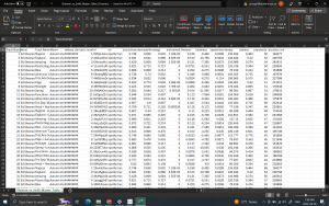
Figure: “Sheeran_vs._Swift_Master_Table(Cleaned).csv”

Dataset Source: https://www.kaggle.com/datasets/jarredpriester/taylor-swift-spotify-dataset

It’s important to note that the datafile ‘Ed_Sheeran_Spotify.cvs.’ contains an error regarding the release date of Sheeran’s album ‘X’ (correct date is November 25, 2012).

Data Provenance:

Both datasets were published and distributed on Google LLC’s open data repository ‘Kaggle’ (an online community of data scientists) that participates in providing online education through free datasets and open collaboration (Wikipedia Foundation, n.d.). While each file was collected and distributed by an individual member on Kaggle, both datasets were generated using Spotfy’s open data source tool: ‘Spotify API.’ By attributing Spotify API as the authoritative data source (and linking the corresponding metadata), each dataset exemplifies proper data provenance standards to be considered reliable for our project.

Data Metrics:

Both datasets contain identical attributes (or ‘metrics’) about the singers’ complete discography. These metrics were further explicated within the corresponding metadata provided by Spotify API (and posted on Kaggle):

  1. Tools Used.
  1. Microsoft Excel: Excel was initially utilized to clean and aggregate our two datasets into a singular (‘Swift v. Sheeran’.csv) file to be later imported into Tableau. The only noticeable limitation of the program was its inability to effectively differentiate and display album titles; numerical album titles were often recognized as integers (instead of a string of characters), and the program entirely failed to recognize Ed Sheeran’s album, titled  “÷” (“Divide”).  
  2. Tableau Desktop: Tableau was subsequently utilized for exploratory and visualization purposes. Once we had a single cleaned dataset to import, Tableau provided the means to conduct our initial research regarding existing correlations between the pop singer’s musicality and popularity. While Tableau allowed us to explore and confirm our initial research suspicions, its major limitation was the program’s inability to provide the aesthetic customization of idioms that we desired. 
  3. Google Slides: Although Google Slides does not provide interactivity with the graphs it does provide us with the ability to customize our exported graphs from Tableau by inserting as many visual elements as was needed over our marks that better expressed their individual items and attributes to the casual viewer.
  1. Analytic steps

STEP 1: Data cleaning (Group Meeting 1):

The first step of the analytical research process entailed preparing the data for effective data analysis. At the start of our research project, we had two separate Excel spreadsheets containing Spotify data belonging to Taylor Swift (‘Taylor_Swift_Spotify.cvs”) and Ed Sheeran (‘Ed_Sheeran_Spotify.cvs.’) – both of which were cleaned and combined into the master excel file. Once the ‘master repertoire’ (consisting of 782 songs shared by the artists) was aggregated in one table, we embarked upon an extensive cleaning process. 

STEP 2: Research and Data Exploration on Tableau (Meetings 2 + 3):

This step entailed a thorough exploration of the recently cleaned data to:

  1. Confirm our initial suspicions that Swift and Sheeran provide a likely musical comparison; and, 
  2. Locate potential divergences within their musical qualities that explain why their career trajectories have so fatefully “divided.” 

From there, we were able to plot the two singers’ comparative streaming popularity over the course of their careers (both across albums and individual song titles). Once we were able to confirm some patterns, our Tableau research took a more refined and goal-oriented approach.

  • STEP 3: Narrative design: 

When beginning to explore our data we knew that Taylor Swift would come out to be the more popular artist overall. However, we also knew that we needed to investigate the data in Tableau to gain a comprehensive understanding of why Taylor Swift was more popular. We were looking to spot the differences in their musical metrics from Spotify to distinguish how each metric related to their overall popularity. What we found was that we were correct that Taylor Swift’s albums are, on average, more popular than Ed Sheeran’s albums. We created graphs that explicitly show each album’s popularity by year and each song’s popularity by year:

Figure: “Album Popularity by Year”

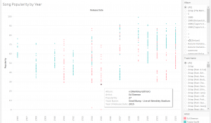
Figure: “Song Popularity by Year”

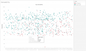
Following this, we made graphs for each metric in the dataset. The metric (for example, danceability) was graphed against the y-axis of popularity and hue coded by singer, for example:

Figure: “Danceability”

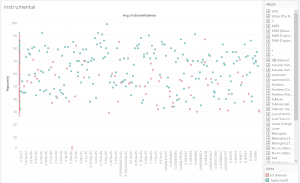
We learned that the individual metrics did not give us as clear of a story as we had assumed they would. Other than, the instrumental quality (instrumentalness) of their songs which had a larger discrepancy than other metrics which could be a factor in Taylor Swift’s overall popularity.

Figure: “Instrumental”

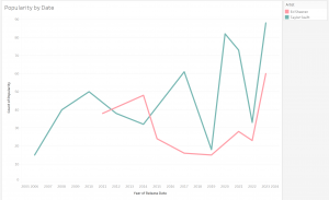
Then, we graphed all metrics by year of release and discovered a description of each artist’s average popularity by year with a line graph to aid the viewer in understanding the continuous nature of their temporal relationships with popularity.

Figure: “Popularity by Date”

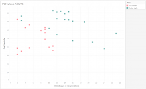
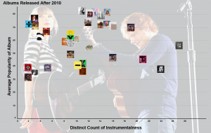
Finally, once we determined the difference in their popularity by year, album, song, and the average of all metrics we filtered our data further to investigate the difference in instrumentalness after 2010 when Ed Sheeran released his first studio album.

Figure: “Post 2010 Albums”

  1. Design Process

After creating the master Excel table “Sheeran_vs._Swift_Master_Table(Cleaned).csv” we began creating graphs. At this point in our data exploration, specificity in design principles was not considered beyond the basic necessity of information communication – for example: Taylor Swift and Ed Sheeran were assigned arbitrary hues for easy visual division between data types. Once we understood the data and our story, it was time to consider the effectiveness and expressiveness when designing the finished graphs (Munzner, 2014). Tableau could have been a fine option to tell our story; however, the lack of interactivity in our ultimate storytelling platform would limit the amount of information that the viewer would have access to which could compromise the graph’s effectiveness. Therefore, the work of creating graphs by hand began. Google Slides allowed for the greatest amount of images and freedom of image placement. 

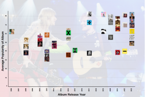
For our graph that represents each album’s popularity by year, we needed to share not only the year, popularity, and the artist’s name but also which album corresponded to each data point. Text description could have been only slightly effective because the labelling technique appeared overwhelming and did not provide enough space for each label to be seen.

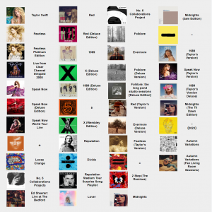
Therefore, we chose to use icons as our marks. Each mark is represented through the iconic use of a specific album cover. There is a legend which clearly shows the album name and cover. Furthermore, the entire graph is laid over a translucent photo of the two singers to provide context, as this communicates race, gender, identity, and the interpersonal relationship between the two singers.

Link to Graphs: https://docs.google.com/presentation/d/16ARxa9z2UPcgGfIoBDJUKK_OS4tXk_Z8mzH3-cS0ldg/edit?usp=sharing

Figure: “Albums by Date (Google Slides)”

Figure: “Albums by Date (Google Slides) Legend”

The same tactic was used to display the average instrumentalness of each album by popularity after 2010.

Figure: “Albums Released After 2010: Popularity and Instrumentalness (Google Slides)”

Figure: “Albums Released After 2010: Popularity and Instrumentlaness (Google Slides) Legend”

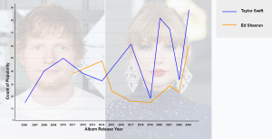
To explore each artist’s popularity over time we opted to display this using a line graph. The line graph expresses the relationship between the metrics of popularity and temporally. The transparent image behind the graph serves two purposes. The first is to show that this graph’s objective is to compare by having two separate photos of the celebrities. The second reason is to reinforce the hue choices of the two artists as Taylor Swift is wearing blue in her photo and Ed Sheeran has orange hair.

Figure: “Popularity by Year ( Google Slides)”

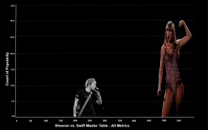
The last graph we produced explores each artist’s overall popularity based on the average results of all the Spotify metrics. This is done through an iconic bar chart on a black background to draw the eye to the two differently-sized figures of Taylor Swift (a larger icon) and Ed Sheeran (a smaller icon).

Figure: “Master Popularity (Google Slides)”

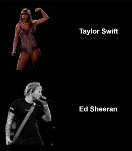
Figure: “Master Popularity (Google Slides) Legend”

6. Describe the story

After playing with the data, we decided to focus on four graphs that helped us discover why Taylor Swift’s music is so good?

Albums by Date

This scatterplot graph displays each artist’s album according to their release year and popularity count until 2024. We measured an album’s popularity by averaging the popularity score from each track. Using their respective cover art to represent each album is an easily discernible way to read this graph at a glance 一 especially for audiences who are fans of either artist.

Here, we can see that before 2014, Swift and Sheeran’s albums had oscillated between the popularity range of 30 to 65. Both Swift and Sheeran released highly acclaimed albums in 2014 一 “1989” and “÷” (“Divide”) 一 which were fairly equal in popularity with scores of 62 and 61, respectively. Although both artists reached higher peaks in the following years, this is the last time they will be comparable in terms of popularity. From 2017 to 2024, Swift’s album’s average popularity consistently stays between 65-85, with only two albums scoring below 57 (“Folklore: The Long Pond Studio Sessions” (2020); and “Reputation Stadium Tour Surprise Song Playlist” (2017)). During this same period of 2017-2023, Sheeran’s album’s average popularity ranges between 38 and 72. It’s also important to note that within this period, Swift has released 16 albums, double that of Sheeran.

Popularity by Year

Our line graph measuring the popularity and release date of Swift and Sheeran’s albums gives us more insight into their careers. We used the popularity averages from each album to measure their overall popularity in the year they were released. If the artist released multiple albums in a year, we calculated the average of those albums. We can identify some divergences between this graph and the scatterplot. For example, if only focusing on albums you’ll see that Swift’s 2017 album “Reputation” is her most popular at a score of 82.8. Yet, in the line graph, her popularity just reaches 60. This is because Swift also released her least popular album, “Reputation Stadium Tour Surprise Song Playlist.” Reading the data this way gives us a continuous and thorough understanding of how the artists compare.

We decided to display this data to give audiences a visualization of each artist’s music popularity over 19 years. We manipulated and displayed the data in two different ways. 

These graphs show that despite there being a time when Sheeran was more popular than Swift, overall Swift has been consistently more popular. 

Master Popularity

For this graph, we wanted to feature the overall scores for each artist and how they compare to each other. We decided to measure their discographies’ cumulative popularity scores against the cumulation of all other recorded metrics. Even from a distance, it’s clear to see that Swift outranks Sheeran in both popularity count and musicality metrics. Sheeran has a combined popularity score of 12, 623 and a combined musicality metric score of 252. In comparison, Swift has a combined popularity score of 33, 266 and a combined musicality metric score of 530. Overall, Swift’s scores are over twice as high as Sheeran’s and this stark contrast is noticeable on the graph thanks to our design choices. They are similar in terms of number of releases], with Swift having released 18 albums and Sheeran releasing 15. Though it should also be noted that Swift debuted in 2006 whereas Sheeran debuted in 2011. 

Overall, this graph does indicate that there is a possible correlation between the musical elements of both artists’ discographies and their level of popularity.

Albums Released After 2010: Popularity and Instrumentalness

Here we are asking the question, could Swift’s popularity be affected by a specific musical attribute?  After going over each metric, we have decided to present our findings regarding the metric of instrumentalness. As previously outlined, the instrumentalness metric is measured by Spotify as a float between 0.0 and 1.0 determining the amount of vocals within a certain track (with 0.0 being none and 1.0 being the maximum).

We decided to visualize albums rather than songs as it would render the graph too crowded to read. We sorted tracks into their respective albums and then accumulated all Instrumentalness scores and assigned that score to the albums. We also chose to compare Swift and Sheeran’s data starting from 2012 as it was the first year where both were actively releasing music. All except two of Swift’s albums had an Instrumentalness score of 10 or higher, with the exceptions both scoring at 3 (“Speak Now (Taylor’s Version)” and “Fearless (Taylor’s Version)”). In comparison, all of Sheeran’s albums score at 11 or below for Instrumentalness. Overall, Swift scores higher across the board with her five most popular albums scoring between 11 to 15.  In contrast, Sheeran’s most popular album, “÷” (“Divide”), is his least instrumental with a score of only 2. Overall, this graph does indicate that there is a correlation between the instrumentalness of Taylor’s music and how it impacts her popularity. 

In conclusion, each of these graphs gives us an insight into both Swift and Sheeran’s popularity throughout their careers. We are able to map their intersections, identify their most/least popular albums, and compare their overall popularity. Our findings show that, especially in the last 5 years, Swift has outscored Sheeran in album popularity, and musical metrics. With further analysis, it would be interesting to explore if Swift’s music success is attributed to her stardom, or vice versa.

  1. Discuss the pros and cons of your designs

Pros: 

  • Using the cover art to represent the album on the graphs was done to promote intuitive reading and visual association.
  • Our use of different types of graphs to show similar data gave audiences a more well-rounded picture of the findings.

Cons: 

  • Our designs were not interactive 

References

Dellatto, M. (2021, December 22). Ed Sheeran’s ‘Shape Of You’ The Most Streamed Song In Spotify History. Forbes. https://www.forbes.com/sites/marisadellatto/2021/12/22/ed-sheerans-shape-of-you-the-most-streamed-song-in-spotify-history/?sh=33796f4875e6

Munzner, T. (2014). Visualization Analysis and Design. CRC Press.

Newman, T. (2024, January 3). Top 10 most-streamed artists of all-time on Spotify in 2024. RouteNote. Retrieved April 9, 2024, from https://routenote.com/blog/most-streamed-artists-all-time-spotify/

Pazzanese, C. (2023, August 2). So what exactly makes Taylor Swift so great?. Harvard Gazette. https://news.harvard.edu/gazette/story/2023/08/so-what-exactly-makes-taylor-swift-so-great/ 

Priester, J. (2024) Ed Sheeran Spotify Dataset. Kaggle. https://www.kaggle.com/datasets/jarredpriester/ed-sheeran-spotify-dataset

Priester, J. (2024) Taylor Swift Spotify Dataset. Kaggle. https://www.kaggle.com/datasets/jarredpriester/taylor-swift-spotify-dataset

Spotify. (n.d.). Get Track’s Audio Features. Web API Reference | Spotify for Developers. Retrieved April 9, 2024, from https://developer.spotify.com/documentation/web-api/reference/get-audio-features

Wikipedia Foundation. (n.d.). Kaggle. Wikipedia. Retrieved April 9, 2024, from https://en.wikipedia.org/wiki/Kaggle

By:

Anna Gibson, Vanessa Matsubara, Lauren Maharaj

Public Art In Vancouver

Team Members: Rachel Zhang, Heather Wan, Fangyi Liu

Link to Our Website

https://fangyiliu2002.wixsite.com/publicart

Our Story

The story that we are telling with our design

The story we’re telling through our designed Information Visualization and website revolves around the vibrant yet often overlooked world of public art in Vancouver and the crucial role local artists play within this tapestry. At the heart of our narrative is the acknowledgment of the challenges faced by local artists—how their work, integral to the cultural and aesthetic fabric of the city, needs greater visibility and support.

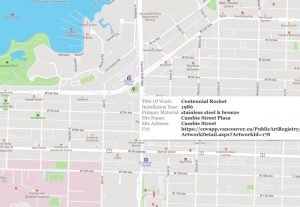
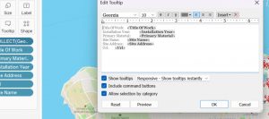
The interactive map at the core of our project does not merely serve as a navigational aid; it’s a gateway to discovery. By cataloging artworks and offering detailed information—such as the title of the work, the year of installation, materials used, and the artist’s name—it invites users to delve deeper into the story behind each piece. This level of detail fosters a deeper appreciation of the art and, by extension, the artists behind them.

Moreover, our project aims to ease the journey of exploration. It simplifies the process of finding and visiting art installations, making the experience more efficient and fulfilling. Whether someone is planning a leisurely stroll through Downtown Vancouver or seeking to immerse themselves in the city’s art scene, our platform empowers them to make the most of their visit.

The narrative we weave is one of connection and support. It’s about creating a link between the community and local artists, highlighting the significance of public art in enriching our shared spaces. Our design is a call to action: to explore, to appreciate, and to support the vibrant art that makes Vancouver unique. Through this project, we aim to not only increase visibility for local artists but also to inspire the community to engage with and champion the arts in their locality.

The objectives of our design

Our goals for this visualization project are to create an interactive map for the users to explore the available public art in Vancouver and to plan the route of their visit based on the basic information about the public artworks. Specifically, our goals aimed to:

Enhance Accessibility: Provide an easy-to-use platform for both locals and visitors to discover and access public artworks in various districts, including Downtown. By visiting our website and interacting with the map, users can view the number of artworks in each area with the option to zoom in for more detailed street-level information.

Detailed Artwork Information: Enable users to access detailed information about each artwork by clicking on the red icons on the map. This information includes the Title of Work, Installation Year, Primary Material, Site Name, Site Address, and the artwork’s URL, assisting users in making informed decisions about which artworks they wish to visit.

Optimize Visit Planning: By categorizing and displaying the number of artworks by region, our design supports users in selecting districts to visit based on the density of artworks. This feature aims to maximize the efficiency and fulfillment of their journey, allowing for a more organized and enriched exploration experience.

Design Process

Prepare Stage 

Sketching

Before we start, we have a meeting about what we actually want to create – a map. So we first drew a sketch about that, including the location of each artwork and the number of artworks in that neighborhood. Based on what we learned in class, we think this kind of visualization is expressive and effective.

Data Sets

The details of the data set we used

We use two datasets as the source of our project.  We choose the “CSV Whole Data Set” and “GeoJSON’ ‘ from the open data portal on the website “City of Vancouver”. The “CSV Whole Data Set” dataset provides detailed information on public art installations across Vancouver, including the art’s location (site address and neighborhood), description, artist and their nationality, installation date, installation status (whether in place or no longer in place) and general features of the artworks such as the type of the artworks and materials. The dataset is comprehensive, updated weekly to reflect new additions or changes, and includes coordinates for mapping, which are used for creating the Geographical map in Tableau. The “GeoJSON” dataset serves as a resource for exploring the detailed and precise location of the artworks. 

The tool we used to transform the data into an information visualization and rationale for using it 

We mainly use Tableau Desktop’s Data Source interface to clean the data and combine it with Tableau Desktop to create the information visualization of the dataset of public artworks and artists in the Greater Vancouver Area. Our goals for this visualization project are to create an interactive map for the users to explore the available public art in Vancouver and to plan the route of their visit based on the basic information about the public artworks. As we’ve learned in creating a geographical map, location information such as coordinates and zip codes can be identified by tableau and transformed into the markers on the map. Tableau is the most intuitive and easiest interactive mapping tool available. 

Data Cleaning

At the beginning of our discussion, we wanted to include as much detail as possible about various artworks, such as the artist’s statement, the artist’s ID number, etc. We thought our perspective on some of the information might change during the process of data visualization in Tableau, so we didn’t delete any data in Excel. Instead, after importing the data into Tableau, we hid columns that seemed unnecessary as the data visualization progressed. This way, if we need the data later, we can simply unhide it. Additionally, we made some titles in the original file more concise to improve aesthetics, such as changing “StatementofArtist” to “Artist Statement,” even though we ended up not using this column.

Visualization Process

After hiding and filtering the data, we started to create our first worksheet, a map named In Place. We dragged the Geometry, Title of Work, Primary Material, Installation Year, Site Address, URL, and Site Name into the Marks section.

To offer our users detailed specifics for each piece of art, including the Title of Work, Primary Material, Installation Year, Site Address, URL, and Site Name, we realized the order should prioritize the Title of Work. Initially, the sequence in Tableau was not orderly, prompting us to utilize the Tooltip function for a new arrangement and organization of the sequence, enhancing our users’ ability to access information in a more logical and user-friendly manner.

For the map feature, we chose a colorful map background to enhance the visual appeal of our visualization (Select Map > Map Layers > Style FYI: https://help.tableau.com/current/pro/desktop/en-us/maps_options.htm). We designed it to resemble popular mapping services like Google Maps, aiming to provide a familiar and easy-to-use experience on our website. The shape of the coordinate markers was customized with an image of a red marker we found online and added to Tableau’s icons (We created a folder with our custom icons, and then we pasted the folder into the Tableau folder named “My Tableau Repository” and clicked Reload Shapes button FYI: https://www.tableau.com/drive/custom-shapes). The positioning of each art piece’s location was determined using latitude and longitude data from a GeoJSON file. 

We prioritized showcasing art pieces marked as In Place, believing this would optimize the relevance of our information. By adding Status to the filters and choosing only the In Place option, we tailored the display to include these specific artworks. Anticipating a future need for information on artworks not currently in place, we created a duplicate of this sheet. In the duplicate, we adjusted the filter to display only those pieces categorized as No Longer In Place.

Next, we embarked on developing bar charts to visualize the quantity of artworks within various regions. A new worksheet titled “Geo Local Area” was established for this purpose, where Site Address, Status, and Geo Local Area were added to the Filters. The Status filter was specifically set to include only artworks identified as In Place. The Site Name was assigned to the color feature with a choice of a green palette, and it was also inserted into the Labels for clarity. The layout was organized with the Site Name designated for Columns and Geo Local Area for Rows.

In our final step, we focused on providing a user-friendly interface. Therefore, we created a dashboard that merged the sheets for In Place artworks and Geo Local Area. This amalgamation led to the completion of our final Visualization.

And we design an interaction, when users click on each region, it will display only the number of artworks and detailed information for that specific area.

Website Design

Our website excels in visual variety, simplicity and intuitiveness of page design, and narrative integrity. We focused on clean page design, aiming to highlight the interactive map as the visual centerpiece. In the interface design, we Integrate elements of Vancouver’s cityscape or indigenous art, to give the site a unique and culturally relevant aesthetic. 

In terms of the website’s use of visual diversity, we feature not only a comprehensive map of the Greater Vancouver area but also detailed maps of specific neighborhoods like Downtown and Mount Pleasant. Users can navigate to these detailed maps without following the narrative order to scroll down, by clicking buttons on our site, showcasing the diversity and the convenience of our visualizations. The interactive map on our website supports user-initiated zooming in and out, offering a detailed view of public art installations. Users can hover the mouse over each coordinate to access basic information about each public art piece, enabling an interactive and informative exploration of art in the area. 

Additionally, our homepage includes a text introduction and a “more info” section, listing third-party websites to encourage further exploration of public art, thus enriching the narrative completeness and integrity of our webpage, making it a comprehensive storytelling platform. 

For our general website creation process, we begin by using the web-design platform Wix. We then focus on crafting interactive elements to engage our audience, followed by writing an introductory section that outlines the site’s purpose and a “more info” section that is directed to other third-party resources. Next, we integrate Tableau visualizations by embedding the code into Wix, ensuring the data is displayed effectively. Finally, we meticulously adjust the details, optimizing the layout and design to enhance both the visual appeal and functionality of our site.

Additionally, considering that our website might be used while people are traveling, we also made it allow mobile access. The mobile view allows users to open the webpage to view searches anytime and anywhere when they are out and about, increasing the flexibility of our visualization.


You May Ask

How did we make sense of the data to create our visualizations?

Our team aimed to include as much detail as possible about various artworks for the visualization, focusing on details like the artist’s statement and ID number. They imported data into Tableau without deleting any, choosing to hide unnecessary columns during the visualization process. This approach allowed them to adapt their visualization as needed without losing any initial data.

Did we explore the data visually to find interesting patterns that later became our final visualizations?

Yes, the process involved creating an initial map worksheet where various data points such as Geometry, Title of Work, Primary Material, Installation Year, Site Address, URL, and Site Name were dragged into the Marks section. This step, along with prioritizing artworks marked as “In Place” and developing bar charts for visualizing the number of artworks within various regions, indicates a methodical exploration of the data to discover and emphasize significant patterns.

Did we know the argument or idea to be communicated right from the beginning, and we focused on presenting the data/evidence to communicate it visually?

Our group’s primary idea was to create an interactive map to help users explore public art in Vancouver and plan their visit routes. This goal was clear from the start, guiding the visualization process. The team focused on presenting data that would enable a user-friendly experience, emphasizing artworks “In Place,” optimizing the relevance of the information provided, and tailoring the visualization to ensure it was both intuitive and practical for users to navigate. Our visualization project was guided by the initial objective to make public art in Vancouver accessible and navigable for users, with a clear focus on enhancing user interaction with the data. The team’s approach to data preparation, exploration, and visualization was strategically aligned with this goal, employing tools and techniques in Tableau to effectively communicate the intended message.

Our Review

The pros and cons of our designs to tell a story based on data or to derive analytical insights

Pros: Our designs effectively utilized clear, concise maps that directly served our core objective of enabling users to explore public art in Vancouver. By dividing the artwork by regions and providing detailed information such as the artwork’s exact address, we significantly improved the usability and aesthetic appeal of our visualizations. This design choice not only facilitated a more engaging user experience but also underscored the visual appeal as a pivotal component of our project. The aesthetic design was not merely an afterthought but a deliberate strategy to enhance user interaction and engagement with the visualized data.

Cons: Despite these strengths, our designs faced several challenges. One major issue was the incomplete data; for instance, the absence of specific addresses for some artworks introduced gaps in our map’s comprehensiveness. The differentiation between artworks that were “In Place” versus “No Longer In Place” prompted considerable discussions within our team regarding the inclusion of the latter. These discussions revealed a deeper concern about how filtering options might affect the visual appeal and the relevance of displaying artworks no longer present to our users. Such artworks, while no longer physically present, remain integral to Vancouver’s art narrative. Balancing the aesthetics of our visualizations with the inclusivity of all relevant data emerged as a critical consideration. Future endeavors will need to navigate these complexities, striving for a design that marries beauty with a comprehensive data narrative.


Our observations about the strengths and weaknesses of the tool(s) in relation to our task and the data

Strengths

Clarity and Simplicity: The tools allowed us to create clear and simple data visualizations that communicated our message directly and effectively. The logical structure of the tools facilitated a straightforward design process, enabling us to meet our objectives efficiently.

Strong Logical Framework: The inherent logical capabilities of the tools we used, such as Tableau, were instrumental in organizing and presenting the data. This aspect was particularly valuable in managing and filtering vast datasets, ensuring that the final visualizations were coherent and aligned with our project goals.

Maximized Achievement of Objectives: Through the use of these tools, we were able to maximize the realization of our project’s aims. The functionalities provided by the tools supported our tasks, from data cleaning to the creation of interactive maps, allowing us to achieve a high level of precision and relevance in our visualizations.

Weaknesses

Limited Aesthetic Options: While functional, the tools offered limited options for enhancing the visual appeal of our visualizations. The basic set of images and icons constrained our ability to infuse creativity and innovation into the designs. This limitation was a significant drawback, as a more attractive and engaging presentation could potentially improve user engagement and the overall impact of our project.

Need for Greater Creativity and Innovation: The tools’ constraints on visual elements highlighted the need for greater creativity and innovation in our visualizations. Expanding the range of visual customization options, including images, icons, and overall design aesthetics, would significantly enhance the ability to create more visually appealing and engaging visualizations.

Future Implement

The decision to not include a section on the type of artwork in the website for users to explore is primarily based on our current stage of development and priorities. Our focus has been on ensuring user accessibility and providing a seamless experience for tourists and other users. While we acknowledge the potential benefits of including a “type” feature to enhance the exploration of Tableau’s functionalities in the future, it is a new concept and functionality that cannot be implemented at this stage. Our website already fulfills all aspects of our storyline and meets the immediate needs of our users. However, we remain open to future improvements and innovations, including the incorporation of a “type” feature, as we continue to refine and enhance our visualization platform.

Citation Page

Dataset

City of Vancouver. (n.d.). Public art. Retrieved Apr. 8 2024, from https://open data.vancouver.ca/explore/dataset/public-art/export/?location=12,49.26097,-123.13232

Web design

Create A Stir. (n.d.). Luke Parnell: Indigenous History in Colour at Bill Reid Gallery. Retrieved Apr. 8 2024, from https://www.createastir.ca/articles/luke-parnell-indigenous-history-in-colour-bill-reid-gallery

Our city. our art. our Vancouver. (n.d.). Our City. Our Art. Our Vancouver.

https://ourcityourart.wordpress.com/

Vancouver, C. O. (n.d.). Artist opportunities. City of Vancouver.

https://vancouver.ca/parks-recreation-culture/opportunities-for-artists.aspx

IT application. (n.d.-b). https://covapp.vancouver.ca/PublicArtRegistry/

Causes and Stigmas of Obesity in Mexico, Peru, and Colombia

Nil Tekin, Haolin Wu, Michael Wu

Links to Information Visualization Products

  • Infographic

https://www.canva.com/design/DAGBsay4vLQ/dpjVXr1SskszBd70XCP02g/edit?utm_content=DAGBsay4vLQ&utm_campaign=designshare&utm_medium=link2&utm_source=sharebutton 

Background Information/Context

Obesity is a disease that can be classified as excessive body fat, and may lead to a variety of other health issues (Cleveland Clinic). The causes of obesity are complex, and may be related to genetics, poor mental health, other illnesses, and certain medications (Cleveland Clinic). Repeatedly, high obesity rates have been linked to foods with ingredients that contain high fat, salt, and sugar. There are different types of obesity that are used to classify people by the severity of the illness. Class 1 contains a low risk of obesity, with a BMI between 30 to 34.9, Class 2 is moderate risk with 35 to 39.9, and Class 3 is high risk with 40 or more BMI (MedlinePlus). 

In particular, obesity in North and South America is a rapidly growing issue that is affecting the lives of millions around the world. According to Simón Barquera and Juan A. Rivera, this issue has been prevalent in Mexico for the past 30 years, mainly caused by a change in diets due to economic growth, from natural ingredients to more processed ones that have a high fat and sugar content. In Peru, a significant percentage of the population is obese due to unhealthy diets and decreased exercise (Peru Telegraph). In Colombia, economic issues and poor lifestyle choices have led to significant rates as well (Betancourt-Villamizar et al.). 

Usually associated with adults, obesity is beginning to affect younger people more than ever. Obesity is an illness that particularly contains not only scientific but psychological layers as well, making it an interesting topic for visualization. We are able to then detect certain trends and connect them to other health conditions and behaviors, such as genetic influences.   


Objectives

In this project, our intended goal was to understand the nuances of obesity from three regions: Mexico, Peru, and Colombia, and demonstrate the severity of the illness. With our visualizations, we hope to garner attention onto the illness, to inspire more self-care and healthier lifestyle choices. Our intended audience are adults who are not underweight, as well as older teenagers. Showcasing that obesity is closely related to one’s genetics will hopefully reduce the stigma that exists in society. With our visualization on body weight and exercise, we also wanted to demonstrate that not all obese people are “lazy” and do zero exercise within a week. The rest of our visualizations focused on discovery, including the correlation between age and weight, and eating habits. 


Dataset Details 

The dataset that we used included information collected from Mexico, Peru, and Colombia. It was very rich with the amount of attributes it contains, which is necessary for such a complex topic as body weight. For example, the age, gender, height, family history of obesity (yes or no), and Body Mass Index (BMI) attributes allow us to get detailed insight into each row that represents an individual. Interestingly, not every row contains data from individuals who are obese, referred to as Normal_Weight, and it includes people classified as just overweight as well, at 2 different levels. 

BMI calculation field was created by us when cleaning the data in Excel, and was not originally included within this data source. It was made by dividing their weight in kilograms by the square of their height in metres, based on the metric system.

BMI formula 

This calculation was done to allow us to have more freedom to creatively experiment with the attributes on Tableau Desktop.  

Tools Used

The main tool that we used to transform our data into an information visualization was Tableau Desktop. As a flexible interface, we could creatively manipulate datasets to convey a story. Selecting certain categories also highlights one and dims others, which allows users to focus on a single aspect at a time, which is helpful when graphs and their marks and colors start to become overwhelming to the eye. The user is also able to select many different types of marks from a list that Tableau provides, which allows for experimentation with visualization preferences. 

As for the weaknesses of Tableau, an issue may arise during the creation of calculating fields. If one does not have past experience with coding, they may not be familiar with how formulas work for their visualization. The data must also be carefully cleaned beforehand to avoid errors that the system may not be able to recognize. We had to handle our dataset carefully before proceeding, and plan what attributes we were going to include. 

Canva was used as a creative graphic design platform to craft our infographic, containing information about the findings of our visualizations, with the data collected by F.M. Palechor and A.H. Manotas. Images were used in the composition as a tool to catch a viewer’s attention and compliment the findings about obesity. 


Analytic Steps

As obesity is a very broad topic, when exploring our dataset on Excel and Tableau Desktop, we initially did not have a distinct idea of what story we wanted to tell with our visualizations. We took some time to think about what arguments we wanted to make. First, our intention was to focus on obesity rates within British Columbia, and found a dataset to provide us with the information. However, it was apparent that drastic levels of obesity trends were not detected within the region, compared to other parts of the world, where it is becoming a more widespread issue even for children. Finally, we found a journal conducted by Fabio Mendoza Palechor and Alexis de la Hoz Manotas, with data that they collected from people within three Latin American countries. Their focus was on two aspects that were associated with causing obesity, eating habits and physical conditions. 

With our cleaned data, we had almost 20 attributes, and decided to exclude some of them from our focus, such as the “NObeyesdad” category that placed individuals into different weights. A confusing entry under this was “Insufficient_Weight”: did this mean the person was underweight? The article mentions it as well, and perhaps labeling them as underweight instead may have been a clearer choice, for the reader to understand better. 

This first report presents a comprehensive analysis of the correlation between obesity and family history, drawn from a study that categorized subjects into six weight classes: underweight, normal, overweight, and obesity classes 1, 2, and 3. The visual representation of data showcases a strong positive correlation between family history and the incidence of obesity, with a higher proportion of subjects with a family history of obesity being found in the higher obesity classes. Among individuals categorized as overweight, 83.6% have a family history of obesity. This percentage rises distinctly with the severity of obesity: 98.1% in Obesity 1, 99.7% in Obesity 2, and 100% in Obesity 3. A significantly lower percentage of individuals with underweight and normal weight report a family history of obesity.

The data visualization showcases the influence of genetics on body weight. The ascending trend of family history prevalence with increasing obesity categories suggests that obesity is not solely a product of lifestyle choices, but rather a complex trait influenced by genetic makeup. There exists a stigma that associates obesity with laziness; however, our findings emphasize that obesity is frequently linked to factors beyond individual control, such as genetics. Recognizing the genetic component in obesity is essential for fostering a more empathetic and scientifically informed public attitude.

In our study, information visualization serves as a crucial tool in uncovering the nuanced relationship between obesity and family history. Interestingly, it also highlights that a substantial proportion of underweight and normal-weight individuals—45.7% and 54.1%, respectively—report a family history of obesity, prompting intriguing questions about the mechanisms of obesity resistance. Despite their genetic predisposition, these individuals do not exhibit obesity, suggesting the presence of other influential factors. This revelation paves the way for subsequent research to delve into the impact of acquired factors such as lifestyle, diet, and physical activity on obesity. The visualization underscores the complex interplay between inherited and environmental contributors to body weight, emphasizing the need for a multifaceted approach to understanding and addressing obesity.

Exploring the relationship between exercise frequency and body weight categories, our graph categorizes subjects as underweight, normal, overweight, and obese. Notably, a lower frequency of exercise is observed among individuals who are overweight and obese. The data shows that 30.8% of overweight and 39.6% of obese individuals do not engage in exercise weekly. Moreover, a considerable portion—43.74% of overweight and 36.7% of obese subjects—exercise only 4 to 5 days per week. In contrast, those in the underweight and normal categories tend to be more active, with the majority engaging in regular exercise each week. Only a small fraction of these groups report not exercising at all. This distinction highlights the significant variance in physical activity levels across different weight categories. 

Research from the Harvard T.H. Chan School of Public Health suggests that many factors affect daily calorie burn, such as age, body size, and genetics, but physical activity is the most changeable and controllable factor. An active lifestyle is essential for weight management and lowers the risk of heart disease, diabetes, stroke, high blood pressure, and certain cancers, in addition to reducing stress. These insights demonstrate the critical need for regular physical activity for the health and well-being of individuals across the entire weight spectrum. From this visualization, viewers may understand that obese people exercise as well, and many times are not suffering from this illness due to a lack of movement and laziness. It should also be noted that not all individuals are able bodied and able to exercise. This visualization should therefore be analyzed loosely, with that consideration in mind. 

Regular physical activities emerges as a key strategy in combating the ‘middle-age spread’—an increase in abdominal weight that tends to occur as people grow older, and which is notoriously more difficult to reverse than in one’s youth. Our study categorized subjects into age brackets of 14 to 30 and 30 to 61, demonstrating a clear shift in weight categories with age. Youth, specifically those between 16 to 26, showed higher instances of normal or underweight statuses. There is a discernible rise in overweight statuses and obesity levels 1 and 2 in the post-30 age group, showcasing the occurrence of weight gain as a natural part of aging. NIH News in Health highlights that losing weight and sustaining physical activity become significantly more challenging during mid-life. This difficulty may be partially attributed to biological shifts, as research by Dr. Jay H. Chung of the NIH has found that an enzyme called DNA-PK can slow metabolism and hinder fat burning. Complementing this, the Harvard T.H. Chan School of Public Health stresses the difficulty of weight loss in later years, advocating for proactive weight management. It emphasizes that an active lifestyle is crucial for maintaining a stable weight, whereas a more inactive life can contribute to gradual weight gain over time. These insights collectively reinforce the importance of preventative health measures and regular exercise to counteract age-related metabolic changes and maintain a healthy weight.

Physical exercise is undoubtedly beneficial for weight management, yet its effectiveness is greatly enhanced when paired with a diet lower in calories. Our graphical analysis indicates a significant positive correlation between obesity and the frequency of consuming high-calorie foods, as well as vegetable intake. The data shows that a high intake of calorie-dense foods is prevalent across all weight categories, with 80.9% of underweight, 73.93% of normal weight, 83.64% of overweight, and a striking 97.74% of obese individuals regularly consuming such foods. The Harvard T.H. Chan School of Public Health reinforces this relationship by asserting that when calorie intake exceeds the amount burned by the body, weight gain ensues. Hence, combining regular physical activity with mindful dietary habits that focus on caloric balance is critical for effective weight loss and long-term weight management. This may allow for viewers to understand the importance of healthy choices of consumption, and which food group should be preferred. However, it must be noted unfortunately that not everyone is able to afford healthy foods, and have no choice but to eat fast food that contains ingredients of lesser qualities.  


Design Process and Principles

With our cleaned data, one of the first visualizations we experimented with on a worksheet on Tableau was corresponding age and weight. We were able to quickly see that the ages between 18 and 27 had the highest rate of obesity. This was surprising, as they are assumed to be more active compared to people who are further in their adulthood. 

An infographic was created on Canva to showcase the findings of our visualizations. We used a template to support the creation of the layout of the infographic, and then tweaked everything else to make it our own. The aim of this article was to transfer our findings onto a more visually engaging format, so that more individuals could learn about the complexities and causes of obesity. A section was dedicated to showcasing how genetics play a significant role in cases of this illness, and it should not be brushed off as a person being lazy or making unhealthy eating habits. Another section is about social stigma, to address the greater issues that lead to shaming of obese people, in real life and in the media, connecting it back to genetics as well. Onwards, our next investigation in visualization is mentioned, about physical exercise and obesity, and then about calories in food and eating habits. At first, we did not contain information about our findings, such as overweight and obese individuals having a higher risk of obesity due to their genetics, and added those later to deliver a more refined graphic. Initially, our infographic also only had graphic drawings. We switched them out with our visualization findings instead, to provide direct results of percentages. 

Expressiveness and effectiveness was considered while creating the infographic. For spatial region, negative space was needed to allow the text to be spaced apart, for the readers to read it in a clear manner. A lot of informative text was eliminated, and simple colors were chosen to make it simple and not overwhelming.

Pros and Cons of Designs

A positive aspect of our designs is that our inputs, which create comparisons through visualizations, are very easy to understand for the average viewer, as they relate to the human body. This catches the interest of the audience, as most people already have background information about the causes and effects of obesity due to its presence in popular media. Another aspect that reflects the strong dataset is that it provides extensive dimensions of different variables, from personal background to lifestyles. It covers valuable information that could analyze the cause of obesity and get to know more about obese people’s lifestyle.

However, the dataset itself is also flawed in which the data is not consistent. For example, male participants outnumber female participants, which may lead to biased and inaccurate comparisons regarding gender. Additionally, due to the uneven distribution of data in terms of the categories in BMI, we had to tune our visualization to be related to percentages only. This unfortunately confined our creativity when generating graphs. Lastly, BMI is nowadays considered as not the most accurate way of representing one’s weight in relation to their body. More complex measurements and calculations could be made for future visualizations for a more realistic comparison, which may take more time.   


Works Cited

Barquera, S., & Rivera, J. A. (2020, September). Obesity in Mexico: Rapid epidemiological transition and food industry interference in health policies. The lancet. Diabetes & endocrinology. https://www.ncbi.nlm.nih.gov/pmc/articles/PMC7434327/

Jimenez-Mora, M. A., Nieves-Barreto, L. D., Montaño-Rodríguez, A., Betancourt-Villamizar, E. C., & Mendivil, C. O. (2020, June 3). Association of overweight, obesity and abdominal obesity with socioeconomic status and educational level in Colombia. Diabetes, metabolic syndrome and obesity : targets and therapy. https://www.ncbi.nlm.nih.gov/pmc/articles/PMC7276377/

Obesity: Causes, types, prevention & definition. Cleveland Clinic. https://my.clevelandclinic.org/health/diseases/11209-weight-control-and-obesity

Palechor, F. M., & Manotas, A. D. la H. (2019). Estimation of obesity levels based on eating habits and physical condition. UCI Machine Learning Repository. https://archive.ics.uci.edu/dataset/544/estimation+of+obesity+levels+based+on+eating+habits+and+physical+condition

Summer, E. (2017, June 4). 40% of Peruvians are overweight and obese. PeruTelegraph. https://www.perutelegraph.com/news/peruvian-curiosities/40-of-peruvians-are-overweight-and-obese

U.S. Department of Health and Human Services. (n.d.). Causes and risk factors. National Heart Lung and Blood Institute. https://www.nhlbi.nih.gov/health/overweight-and-obesity/causes

U.S. National Library of Medicine. (n.d.). Health Risks of Obesity: Medlineplus medical encyclopedia. MedlinePlus. https://medlineplus.gov/ency/patientinstructions/000348.htm