Data Acquisition
Step one was to acquire data for the study area. We used three locations for all our data:
- New Zealand Government data
- Canterbury Maps
- Open Street Map
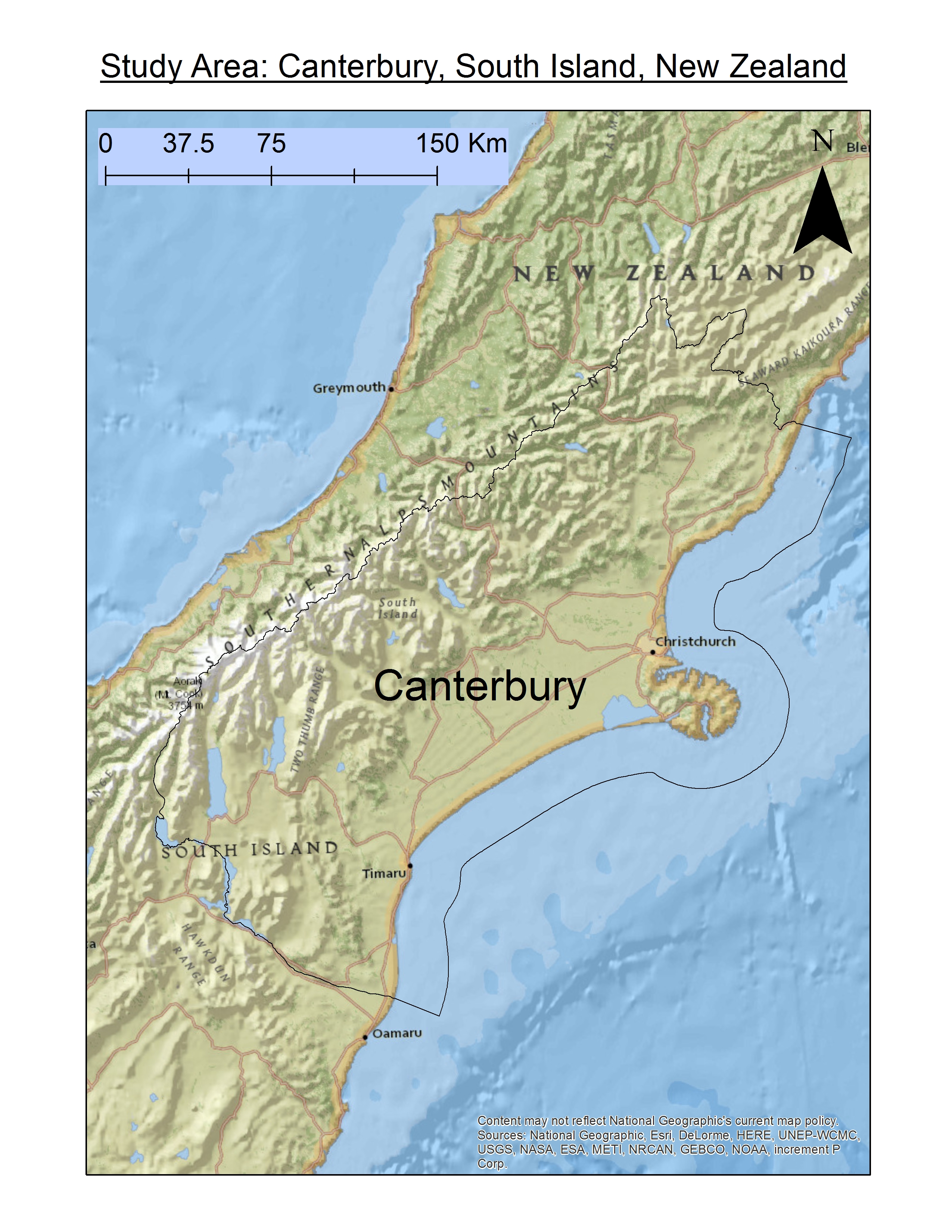
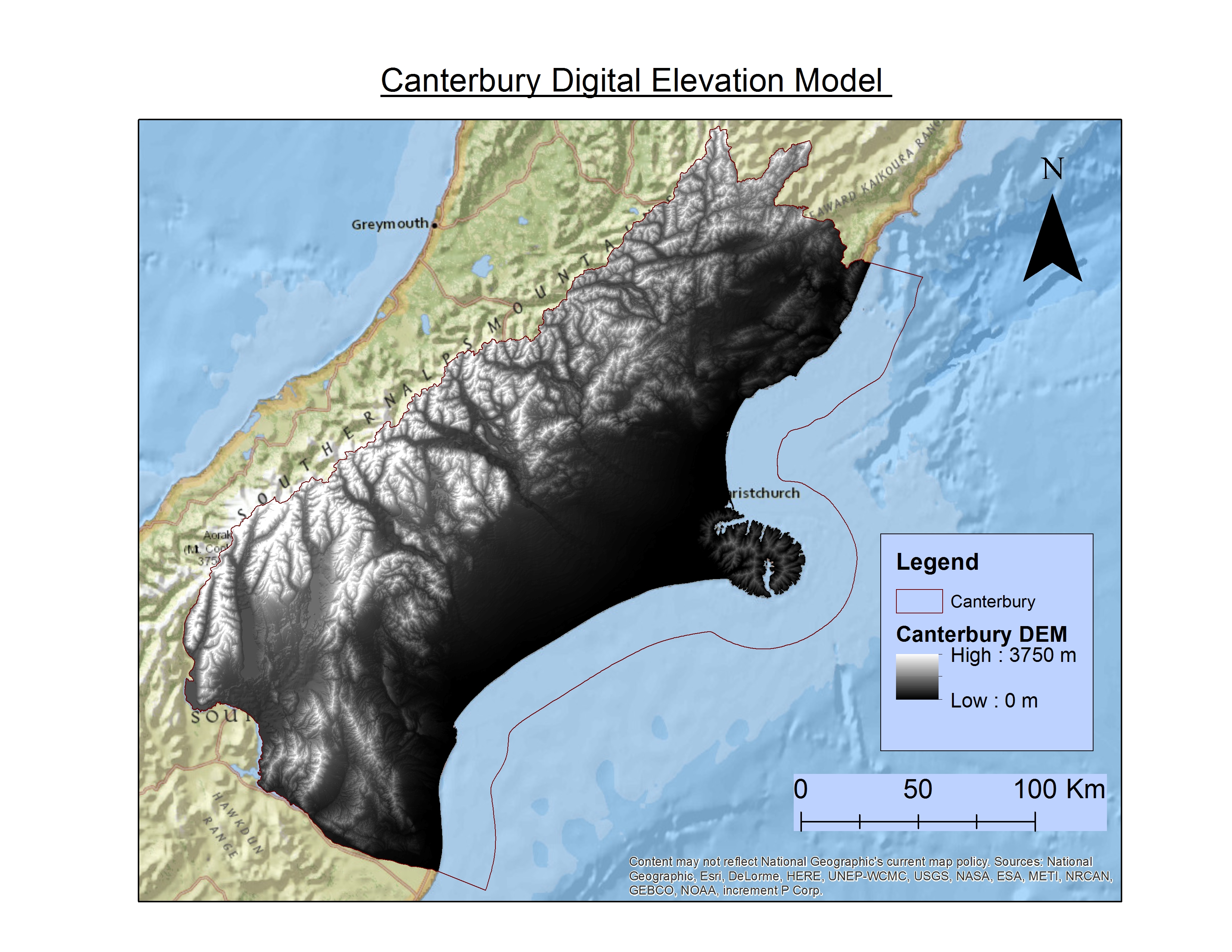
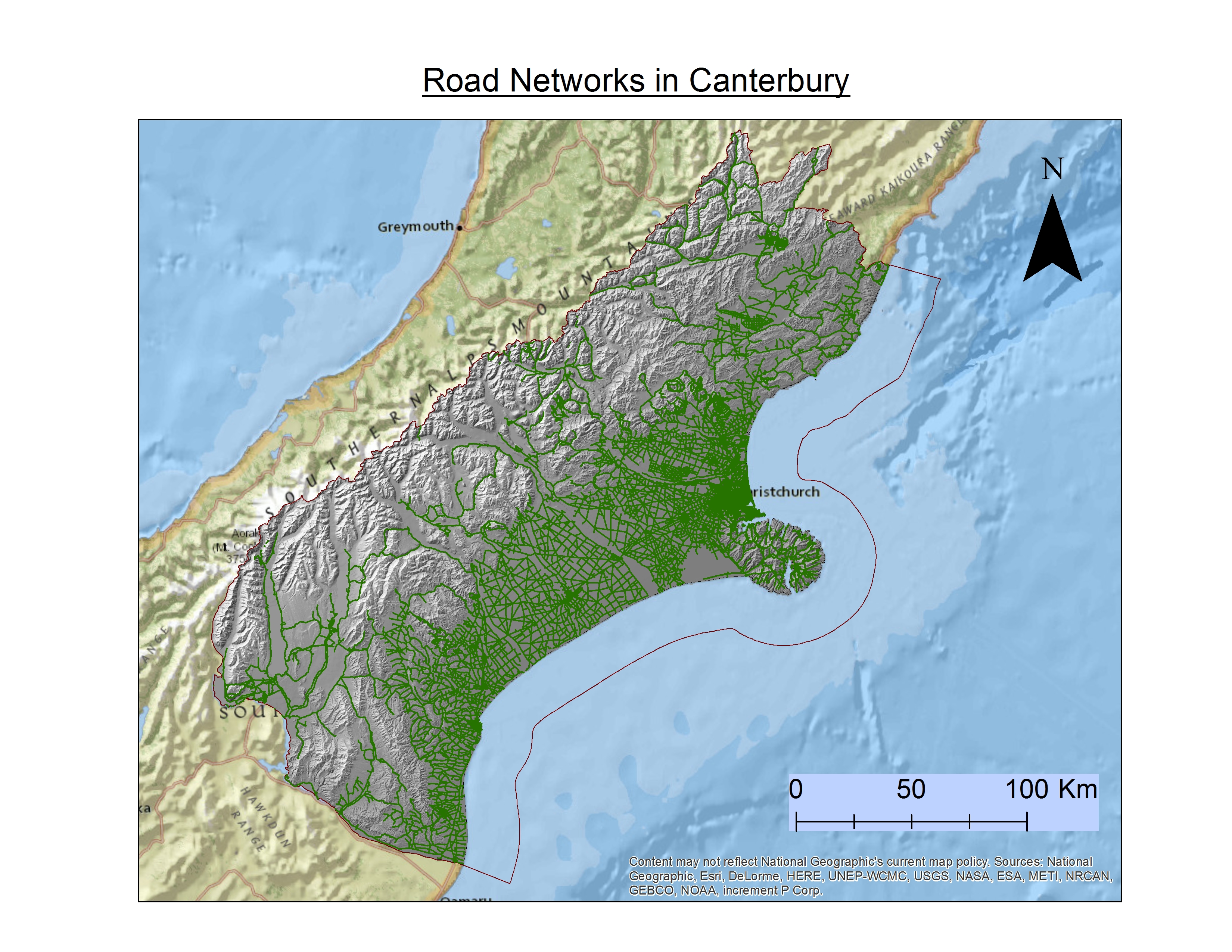
We acquired a DEM of the South Island from the New Zealand Government Data page as well as a shapefile for the districts of the country. The Canterbury Maps website had page after page of data, ranging from public toilets to horse tracks and more. We didn’t end up using much of the data on there, but found some of it useful. Open Street Map provided us with our roads file, because it was the only road file available that had road type data.
Data Set-up and Creation
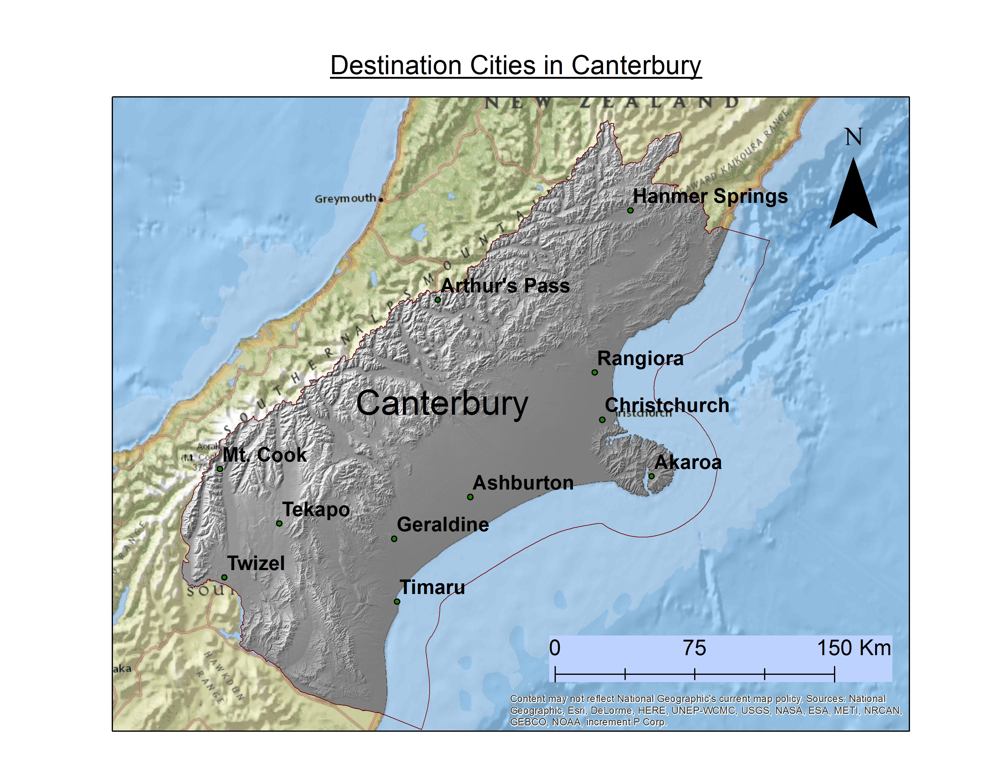
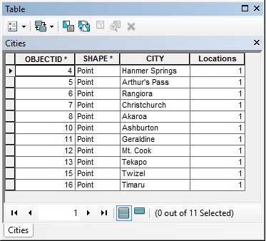
Before we could begin our analysis, we needed to trim our larger New Zealand data down to our specific study area: the district of Canterbury. We isolated the Canterbury area from the districts shapefile, and clipped our DEM raster and Roads shapefile to this extent. Next, we had to create a layer that showed the locations we wanted to visit on our bike tour. With lat/long coordinates gathered from Google Earth, we created point data for each of the ten locations, and saved them in a shapefile within our geodatabase.
Data Manipulation
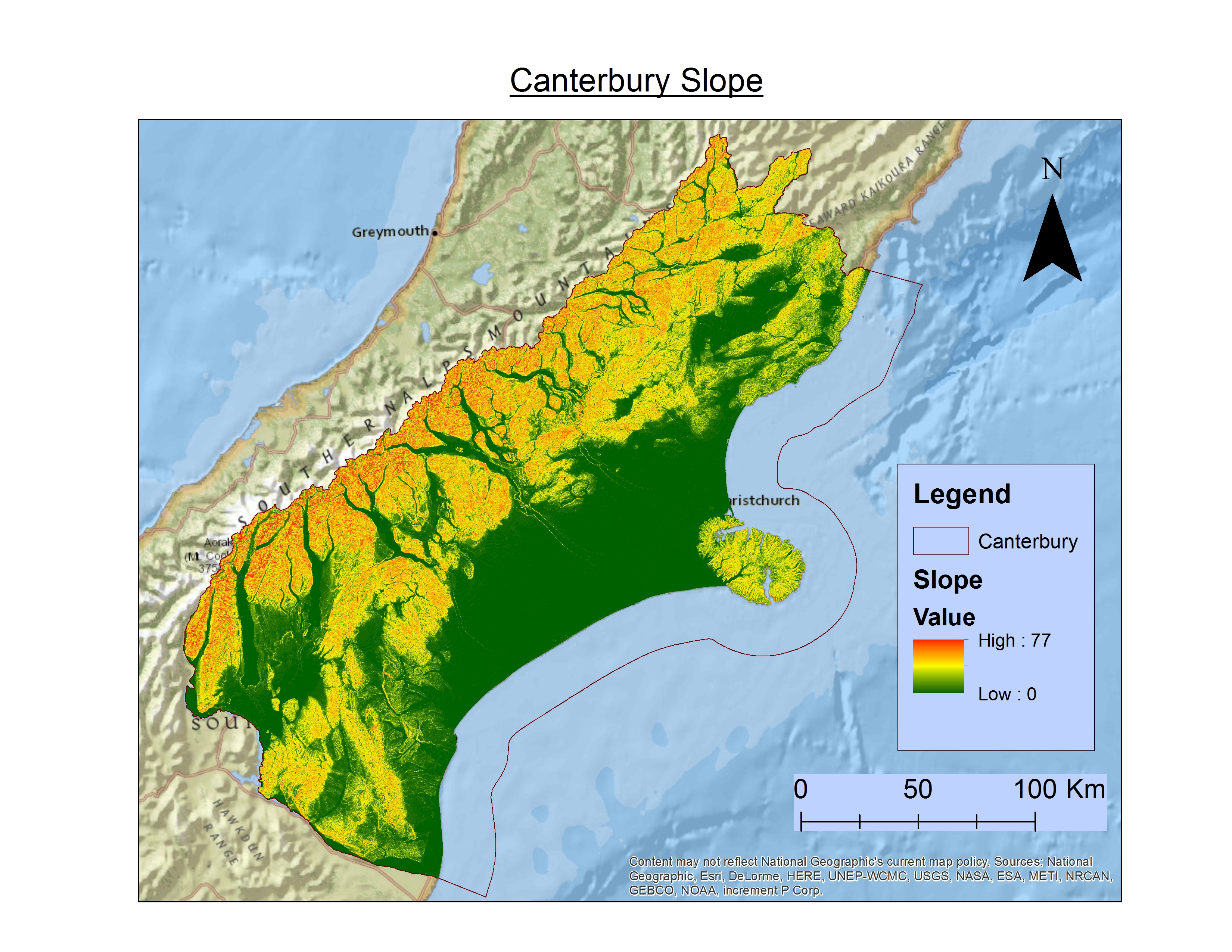
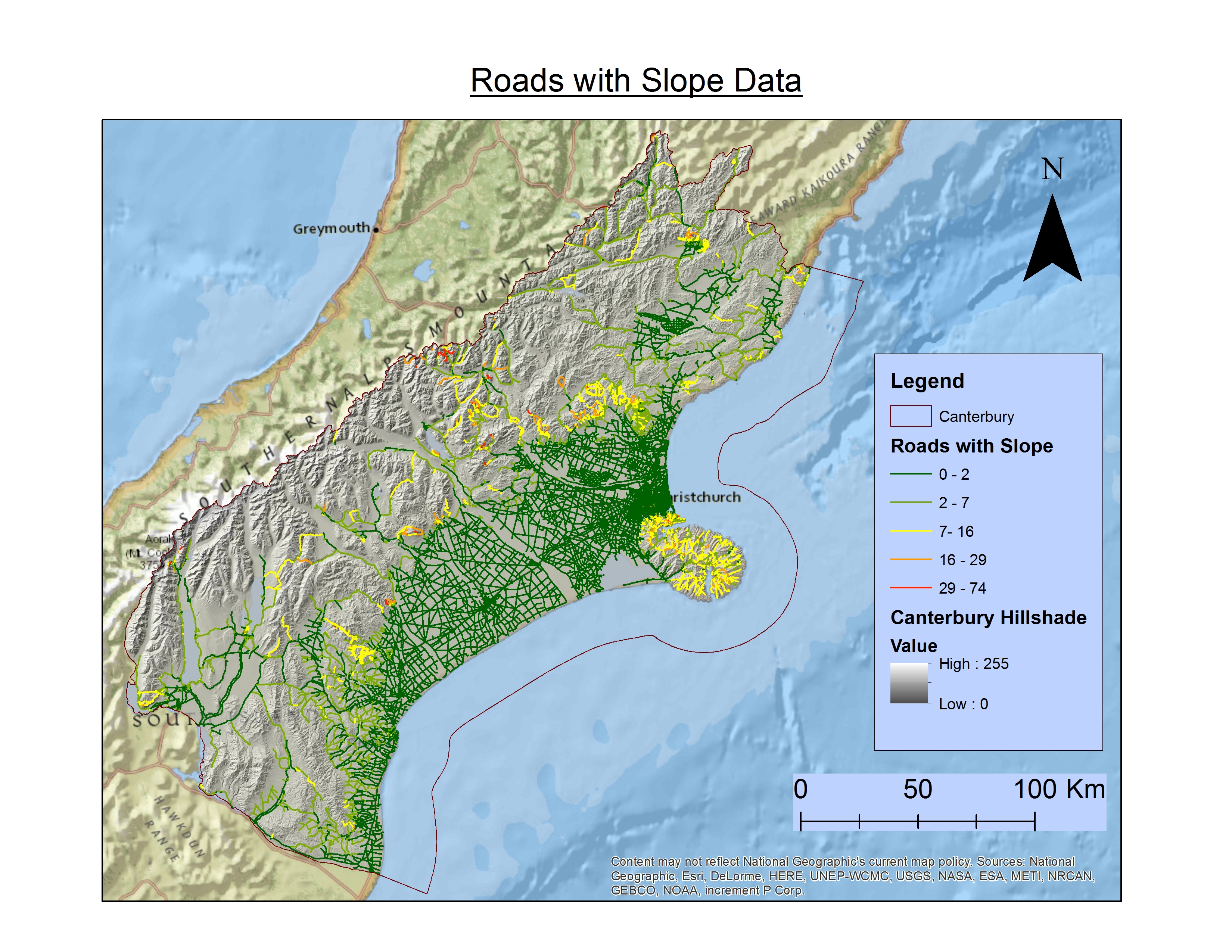
We knew that we wanted to find a route that minimized our elevation change. To gain a better understanding of our study area, we began by creating a slope surface from our DEM, this allowed us to easily see the areas of high and low slope. Following this we used the ‘Add Surface Information’ tool in the 3D Analyst Toolbox, inputting our road file to assign elevation values, as well as calculating an average slope over the given road segment.
Network Analyst
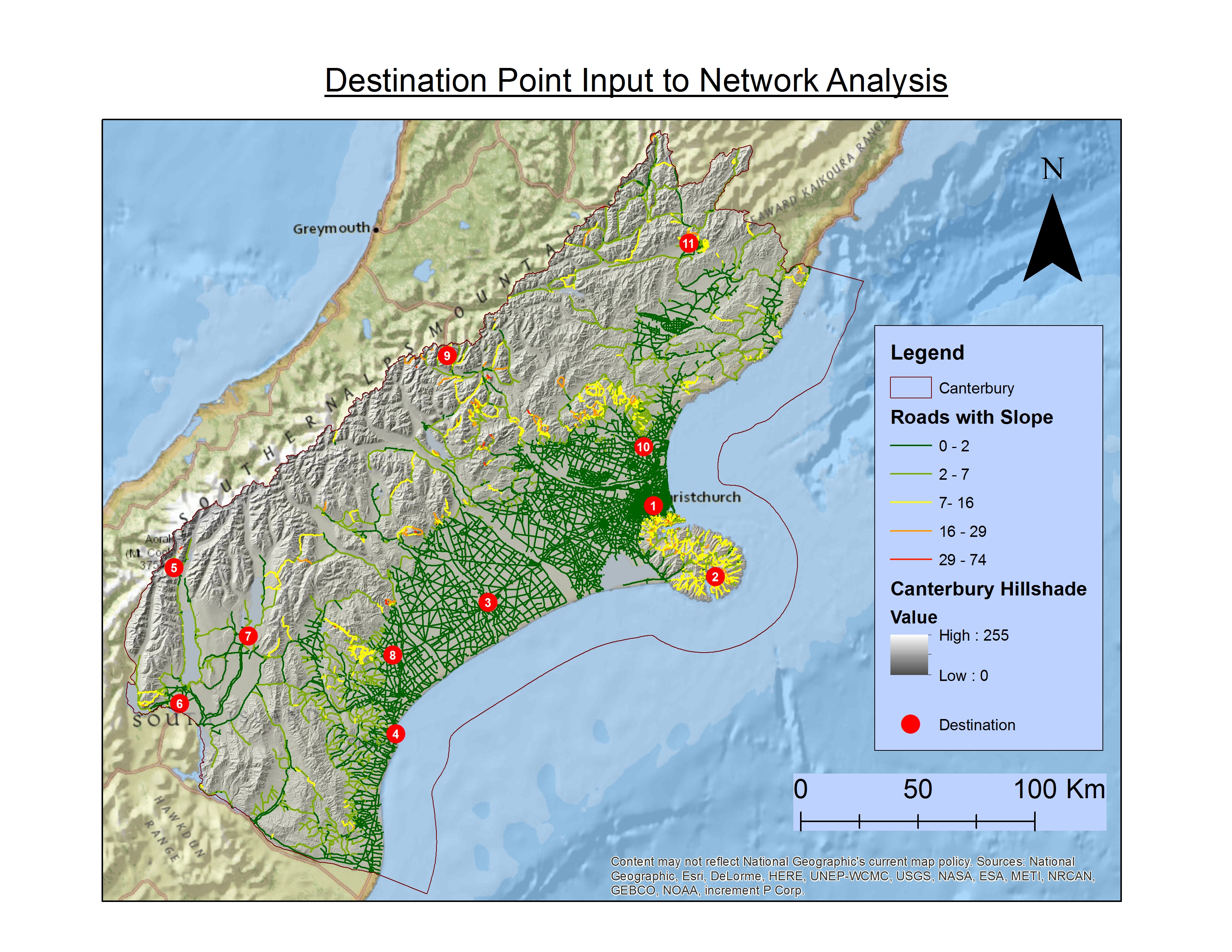
The step that brought everything together also caused us the most trouble. To see a step by step of how we set up a network analysis, click here or see the drop-down menu beneath “methods”. We created two network data sets, one of which used slope parameters to allow us to model the smallest slope change, and the other used length parameters to allow us to model the shortest path distance. To each data set we added 11 stops, one for every destination, and two for Christchurch, as this is the start and endpoint of our route (as the main city in Canterbury, this is the obvious starting point). We then built the two routes, allowing the tool to reorder the stops to find an optimal path. After this ran, we had two outputs. The first was a route that showed us the path that changed elevation the least while still visiting every location, and the second was one which showed the shortest path between all stops, regardless of elevation change.
Unforeseen difficulties
As alluded to above, running the network analysis posed significant complications. While we were successful in creating a route that minimized slope change, and a separate one that minimized path length, we were unable to create one that minimized both these factors. As a result, the minimized slope route does not minimize distance, so it is not the most efficient route distance wise. The network analysis was confused when faced with two paths of equal slope but different distances, and did not have a rule that made it select the shortest route.