
The basis of our spatial analysis falls from there being more variability in crop data than drought data in 2007 and 2014, and within the Kern County. Thus we opted to conduct a spatial analysis of 2014 crops in relation to 2007 crops and 2014 drought conditions. To do this, we first combined the all of the data into one layer and spatially joined 2007 crop data to the 2014 crop data (which includes 2014 drought data). The issue we ran into was attributed from the changes in plot areas from 2007 to 2014. As described previously in Figure Agricultural Plot Comparison in Section Comparison of Data, there is variability in the number of plots in the county and its areas. Thus when we spatially joined the two crop data together using the “One to Many” method, we ran into the following situation:
-
- New 2014 plots that cannot be spatially joined with old 2007 plots (ie. brand new plots) gave null values for 2007 crop data; and
- Old 2007 plots that were removed did not spatially join with the 2014 plot since such a plot doesn’t exist in 2014.
In Situation 1, we assigned the null values an arbitrary value such that the plots still undergo spatial analysis and are not rejected. In Situation 2, since we combined 2007 crop data to the 2014 crop data, any removed 2007 plots were not incorporated into our analysis. As labelled in yellow In Figure Agricultural Plot Comparison in Section Comparison of Data Map, this is a relatively small percentage of agricultural plots that are not incorporated into our analysis.
To run our Ordinary Least Squares spatial analysis the following regression equation was used:
y = b0 + b1x + b2z + ε
(Crop Data in 2014) = b0 + b1(Crop Data in 2007) + b2(Drought Condition in 2014) + error
y = (0.096)x + error
Essentially from our spatially analysis we have found from both our explanatory variables of Crop Data in 2007 and Drought Condition in 2014, only the Crop Data in 2007 is statistically significant (Map 1). From our drought comparison map (Map 2 in Comparison of Data) we found that within Kern County there is little to no variability of drought conditions in the most concentrated agricultural lands. From our agricultural plot comparison (Figure 1 in Comparison of Data) we found a lot of variability from agriculture plots found in 2007 versus 2014. We also found differences in the type of crops planted in 2007 versus 2014 from our crop comparison map (Map 1 in Comparison of Data) and thus the conclusions from the spatial analysis can be valid.
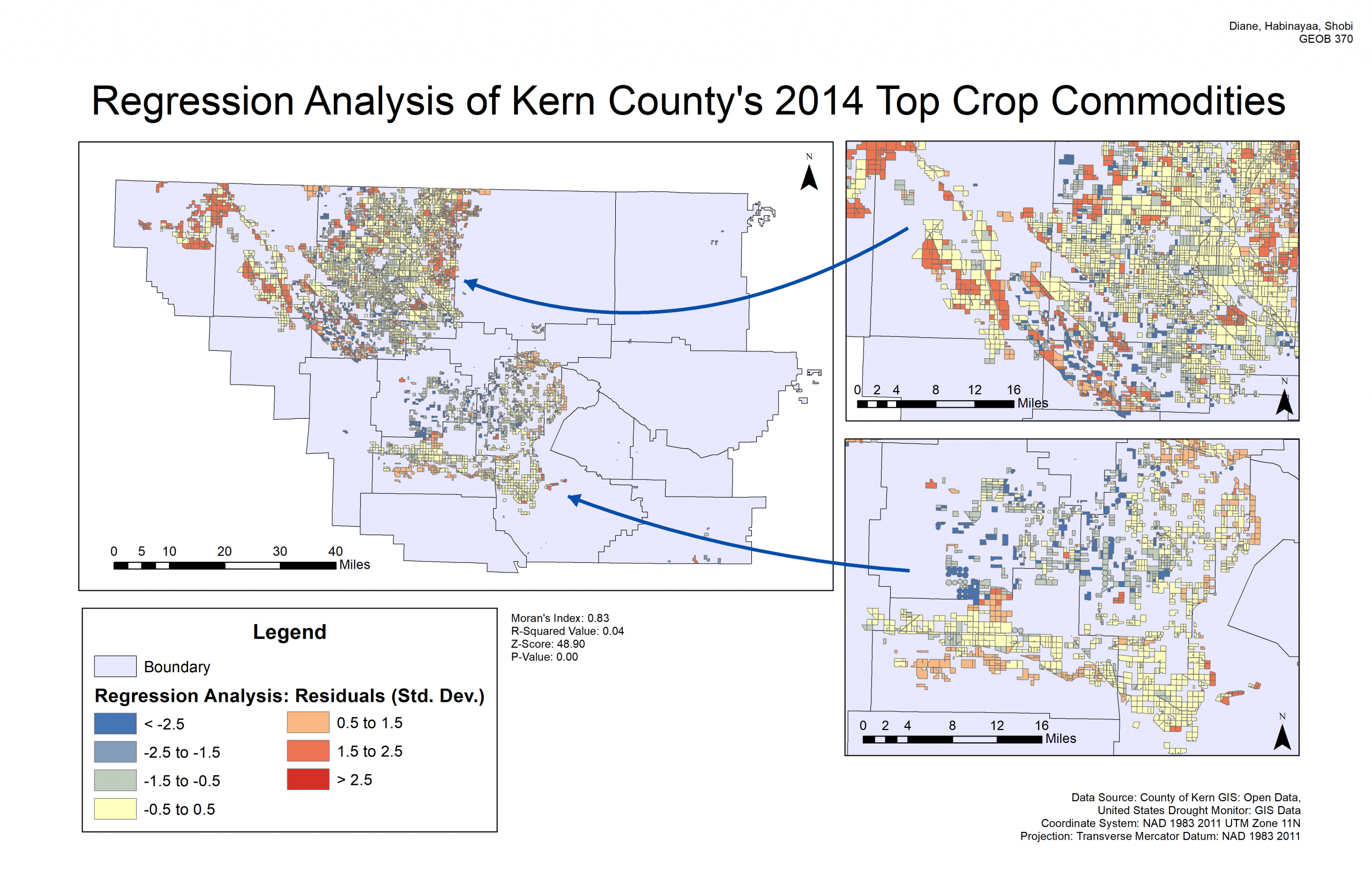
In Map 1 the values retained from our spatial analysis and spatial autocorrelation assessment (Moran’s I) is summarized. Our R-squared value of 0.04 indicates that only 4% of our model is explained by analysis. This result may be plausible as there are multiple anthropogenic factors that can contribute to crop conditions present in 2014. Our Moran’s Index of 0.83 indicates a positive spatial autocorrelation. The z-score value of 48.9 and a p-value of 0 indicates there is a small chance the clustered pattern present in our regression analysis is a result of random chance. This again is plausible, as there are a lot of anthropogenic factors that contribute to what crops are planted where.