Map Distortion and Projection
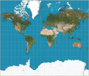
When creating a map in GIS it is possible that the data in the individual layers (a set of data with a common theme) will have been downloaded in different projection systems. Projections are the ways in which a 3D globe is transformed onto the 2D page. The result is always that distortion occurs as it is impossible to perfectly flatten a spheroid. Distortion of area, angle, direction and distance can occur and cartographers must choose which aspect of distortion to accept in order to preserve other aspects (e.g. distort angle, direction and distance in order to preserve area) (see Mercator Projection below).
The result of using different projection systems is that when layers that are projected differently are combined their common features do not align (e.g. the same stream is depicted in two locations). But, ArcMap is able to counter act this challenge with a feature called “project-on-the-fly,” in which features in different projections are temporarily aligned so that they visually correspond (i.e. the stream in two layers would be depicted in the same location).
ArcMap can only project-on-the-fly if the layer is properly referenced, meaning that data about the projection system used is attached to the layer. But, when viewing some layers, their coordinate systems may be described as “unknown.” “Unknown” means that ArcMap does not know the distortion properties and, therefore, cannot align the information in a common projection.
You will know that a layer is not properly referenced if, when you add it to the map, a warning states “unknown spatial reference” and visually the layer’s size, location or shape is different from the existing layers. Alternatively, when viewing the spatial information in ArcCatalog, the current coordinate system is defined as “<unknown>.”
The steps below describe the process of finding improperly referenced data, referencing the data and adding the layers to the map so that features visually align.
Part 1: Review the Spatial Data Properties:
First, you will need to examine the data in ArcCatalog:
- Open Arc Catalog from the start menu
- Create Folder Connection to Data:
- File > Connect to folder > select folder > Okay
- Make sure the catalog tree (the list of information on the main screen) now lists the data you want
Click on each of the layers in turn and view their contents, preview and description by selecting the tabs along the top in turn. The preview will show a map and the description tab will provide some of the meta data from the map, including information about collection and data quality. Read this meta data, paying attention to the coordinate system and extents of the data. Return to the catalogue.
Right click on each of the layers in turn, selecting “properties.” Under the “XY Coordinate System” tab there is a box entitled “Current coordinate system,” this box shows the spatial information of the data. Review the spatial data properties here.
- Note the datum, coordinate system and units used in the shape files. The coordinate system may be a projected coordinate system using meters/kilometers/miles or a geographic coordinate system using decimal degrees
Within the “current coordinate system” box, one or more layers may state “Unknown,” indicating that there is improperly referenced data. Make a note of this layer.
Part 2: Referencing a Layer:
Now, close arc catalogue and open Arcmap from the start menu. From Arcmap it is possible to edit the layers, change their overlay order and fix their spatial references.
When Arcmap opens a dialogue box is opened. Select “templates” from the list on the left and double click on “Blank map.” Arcmap opens with no information displayed.
Launch ArcCatalog from within ArcMap: Windows > Catalog.
Pin the catalogue to the right hand side of the window by dragging the catalog and dropping in to the right. To pin the catalogue, click the push pin symbol on the top right so that it is facing downwards.
In the catalog, find any layers that were not displaying their spatial information correctly in Arc Catalog and right click. Select properties > XY Coordinate system tab. The coordinate system will be listed as “unknown.”

View the box above and navigate to the original coordinate system of the data (selecting a geographic or projected coordinate system, the area you are working within etc.). Click ‘Okay’. Repeat this process for any other layers with improperly referenced data.
Your layers should now be properly referenced with defined coordinate systems.
Now you will need to add your layers to the map’s table of contents to project them all. Find all of the layers you wish to add to the map and drag each in turn to the left hand side of your screen, into the table of contents. You can move the layers within the Table of Contents by dragging and dropping so that all of the data can be seen. The layer closest to the top of your screen will display above all of those below it.
Your layers should now overlay each other and match up, visually aligning due to ArcMap’s “project-on-the-fly” function. But, the project-on-the-fly display does not fundamentally change the projection of the data, it merely aligns common features. Before performing an analysis, you need to change the coordinate systems to a common one, requiring the use of the “Project” tool.
Part 3: Re-Projecting a Layer:
Decide on a common projection system you wish to use, considering the longitudinal extent of your area, its shape and its location.
Open ArcToolbox from the tool toolbar. Move the appearing window to the right hand side of the screen and dock it here. In the toolbox, navigate to Data Management Tools > Projections and Transformations > Project.
In the window that appears type the location and name of the layer you are trying to alter into the “input dataset” box. The output dataset should automatically be filled and the output coordinate system is a projected coordinate system found by navigating to the icon on the right hand side. In the window that appears, select the coordinate system you wish to use. In the case of Canada this is likely the Canada Lambert Conformal Conic for viewing purposes. This projection can found within continental > North America. However, other projections, preserving different qualities may be better suited to other purposes. The “project” dialogue box should resemble the one below:

Press “Okay” and wait for a new layer to be created. This is a new set of data. View the properties window > source. Note the top, bottom, right, left extents and their units. Compare this to the previous layer’s source information. The previous layer can be removed from the table of contents by right click > remove. Repeat this process of modifying the layers into a projected coordinate system for each layer in turn, enabling future data analysis
The map is now ready for analytical use.
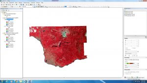
Remotely Sensed Landsat Data:
Can you see change over time in your map? Were you able to find data about the whole globe? Is your map clear to interpret? If not, Landsat imagery may be the solution.
Landsat is a NASA program that is based on satellite imaging. Landsat images cover the whole earth and have been recorded every 16 days since 1972. Landsat satellites are able to take multispectral images, meaning that they are able to show how the world looks in different wavelengths across the electromagnetic spectrum, including wavelengths visible to our eyes (e.g. red, blue, green) and those not visible (e.g. Infrared).
This ability to switch between different wavelengths when viewing Landsat images is a key strength as it enables different features to be identified clearly based on the frequency of reflected light. As a result of using specifically defined wavelength bands, Landsat is able to provide information on land use change, vegetation change, hydrological patterns, urban growth, and more. For example, the Landsat imagery of before and after the Mount St. Helens eruption clearly shows the change in hydrology, vegetation and landform (See Figure Below). Understanding changes and the existing landscape enables people to perform environmental monitoring, track resources and identify future risks to populations (e.x. heighted potential of flooding).
But, more than its ability to filter across the electromagnetic spectrum, Landsat holds three other advantages. Firstly, Landsat images cover the globe, meaning that patterns and trends can be broadly assessed. Secondly, these images are now available for free, making them widely accessible. Lastly, Landsat images have been recorded since 1972, meaning that there is a very long duration of data recorded and slow, longitudinal changes can be observed.
These advantages can be clearly seen in Mount Saint Helens images below build from Landsat Data. They clearly show vegetation and topographical change as a result of the volcano’s eruption.