This week continued on from Week 1’s exploration of key GIS issues and concepts. One key concept that was discussed was scale – not just different size scales, but also different time scales. For example, many natural processes have time scales that extend well into the 100s and 1000s of years, which may be difficult to grasp from a human perspective. As such, it is important to tailor both the spatial and temporal scale to your given phenomenon. We also learned about scale-related terminology, such as grain – the smallest resolution for data and extent – the entire study area.

Autocorrelation

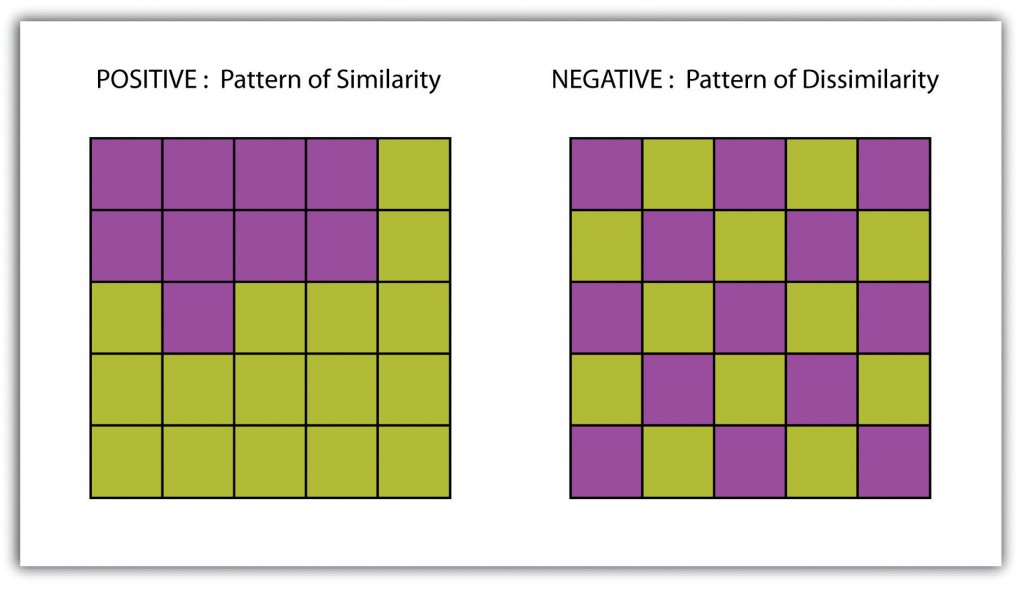
Another important concept is spatial autocorrelation, which refers to the distribution of values in an area. If similar values are clustered close together, for example, they exhibit positive autocorrelation, whereas if dissimilar values cluster together, they have negative autocorrelation. This concept is important because many if not the majority of ecological variables tend to have a pattern of positive or negative autocorrelation.

Gerrymandering

We also discussed the Modifiable Areal Unit Problem (MAUP), which can have a serious impact by distorting data depending on which scale and aggregation one looks at. In particular, we looked at a real world example of MAUP – gerrymandering – which is used by politicians to ensure getting elected by carving out their electoral districts, instead of following logical boundaries (such as a city or a county).