This week saw the wrap up of work on Lab 2, and introduction of statistics. We started off with a review of basic statistics, by looking at measures of central tendency (e.g. mean), variability (e.g. standard dev.), as well as more advanced measures such as skewness and z-score.

We then learned about statistical measures of association, such correlation, cross-tabulation, and regression modeling, which look at relationships between a dependent (response) and independent (predictor) variable.

We look at regression modelling in particular detail, as it is a practical and frequently-used method of analysis. Some of the related concepts we learned about were OLS, collinearity, iid (independent and identically distributed) errors and spatial declustering. We also learned about  geographically-weighted regression,  which is a tool used in ArcMap to account for spatial variance in regression modeling.

Lab 2 Work:

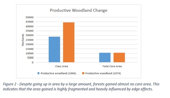
I finished up lab 2 this week, which looks at land use changes from 1966 to 1976 in and around Edmonton, Alberta. The additional variables I chose were Simpson’s diversity/evenness for landscape metrics, and total core area/patch cohesion index for class metrics, with the goal of looking at changes in forested areas in particular (productive woodland).

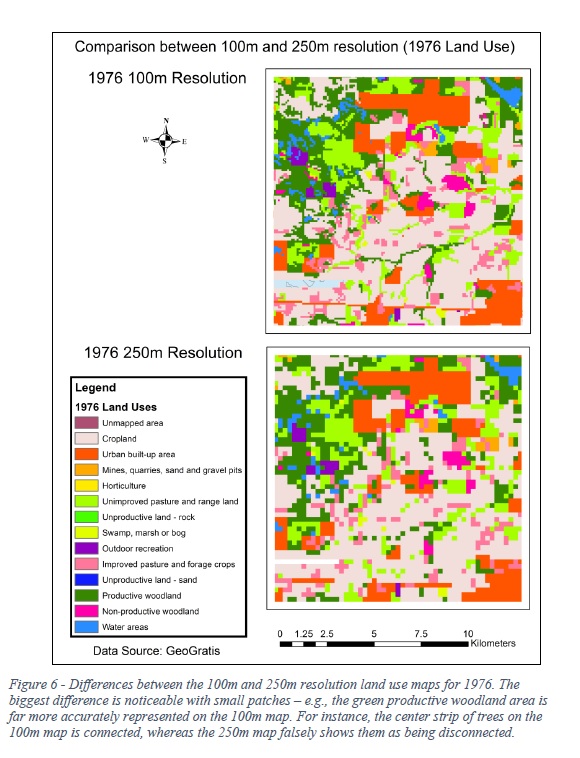
Example Map, showing the differences between the 100 and 250m resolutions:

Example table, showing some of the results of the lab:

This week was spent continuing the work on Lab 2 (analyzing land use changes in Edmonton from 1966-1976) and learning about key landscape ecology concepts.

Landscape ecology is a relatively new discipline which studies landscapes, and more importantly, the relationship between spatial patterns found on landscapes and the related ecological processes. One example used in the class was the spatial pattern of where people with different personality types tend to aggregate in London. For instance, extroverts were far more likely to live in the center of the city, while introverts in the suburbs.

The primary aim of landscape ecology is to understand how ecological processes work and create specific spatial patterns. For example, it would be useful to know why an invasive species has high populations in a specific area, so that we can prevent repeating a similar situation elsewhere. In this case, we can see the spatial pattern – a concentration of an invasive species (like fire ants) – and use that to figure out/understand the process behind it.

An example of a landscape, with basic components studied in landscape ecology, such as patches.

Some important concepts that were discussed this week:

Landscape – “an area that is spatially heterogeneous in at least one factor of interest”

Stationarity (first and second-order) -> a fundamental assumption which supposes that the processes that placement of an object or event do not change over space – differences in values may depend on relative location, but not absolute location -> only works for homogeneous landscapes

Isotropic (no directional bias) / anisotropic (has direction bias)

Process Types:

• Biotic – processes caused by living things (non-human) – e.g. pine beetle infestation
• Abiotic – processes caused by non-living things, such as wind or precipitation
• Human – human impacts, like logging or agriculture
• Disturbances – forest fires, floods, etc

And to close, a couple of interesting ideas/considerations relating to landscape ecology.

Biotic perspectives – thinking like the animal if you’re looking at habitat for example

Criminal perspectives – people tend to commit crimes in areas that fit their socio-economic background – geographic profiling

This week continued on from Week 1’s exploration of key GIS issues and concepts. One key concept that was discussed was scale – not just different size scales, but also different time scales. For example, many natural processes have time scales that extend well into the 100s and 1000s of years, which may be difficult to grasp from a human perspective. As such, it is important to tailor both the spatial and temporal scale to your given phenomenon. We also learned about scale-related terminology, such as grain – the smallest resolution for data and extent – the entire study area.

Autocorrelation

Another important concept is spatial autocorrelation, which refers to the distribution of values in an area. If similar values are clustered close together, for example, they exhibit positive autocorrelation, whereas if dissimilar values cluster together, they have negative autocorrelation. This concept is important because many if not the majority of ecological variables tend to have a pattern of positive or negative autocorrelation.

Gerrymandering

We also discussed the Modifiable Areal Unit Problem (MAUP), which can have a serious impact by distorting data depending on which scale and aggregation one looks at. In particular, we looked at a real world example of MAUP – gerrymandering – which is used by politicians to ensure getting elected by carving out their electoral districts, instead of following logical boundaries (such as a city or a county).