1. DATA GATHERING and PREPARATION

Based on research of habitat preferences, we selected important habitat qualifications for both snapping turtle hibernation and nesting sites. We then obtained corresponding spatial data from a variety of sources, including the Region of Waterloo’s open data site, the Land Information Ontario database, and Geogratis. As referential data, we found Waterloo Regional boundaries, creeks and rivers, wetlands, land cover type, roads, soil types, elevation and elevation points.

We were also hoping to find a dataset of snapping turtle sightings in southern Ontario in order to evaluate the efficacy of our spatial analysis. However, once we downloaded the only existing dataset, we found that the data was too sparse and did not cover most of our analysis area. 

After gathering our data, we formatted it to serve the purposes of our analysis, including re-projecting the shapefiles, clipping them to the study area, and joining/editing attribute tables to make sure that they were ready to be used. For example, our land use shapefile had an attribute table with approximately 20 different land use types! For the purposes of our analysis we needed to simplify them by combining categories into more workable, relevant groups (for example, Treed Swamp, Marsh, Bog, Fen, and Thicket Swamp became reclassified as Wetland, universally conducive to snapping turtle habitat).

We also had to join attribute tables to various soil layer files until we could access the ‘dominant sand fraction’ class on the appropriate soil layer. We chose to use the ‘dominant sand fraction’ class in our analysis because it displayed soils based on the grain size of the dominant sand fraction: coarse, medium, etc. (Snapping turtles typically prefer coarse sand and even gravel for their nesting sites).
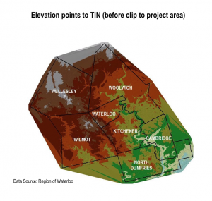
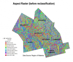
In order to include snapping turtle’s preference for sunny nesting areas, we needed to create an aspect map. We obtained a DEM from the Region of Waterloo’s open data catalogue, created a TIN from the elevation points, and converted it to a raster layer. We then converted this raster layer using the Surface > Aspect tool to create an aspect raster, clipped it to the project boundaries and reclassified it into five directional classes. This way, we could compile the south and southwest facing aspects (the most preferable) together.

 

 

 

 

 

 

 

2. CREATING EUCLIDEAN DISTANCE RASTERS

To ensure that the distance to bodies of water and the distance away from roads was considered in our analysis, we needed to create layers that distinguished between different distances from features.
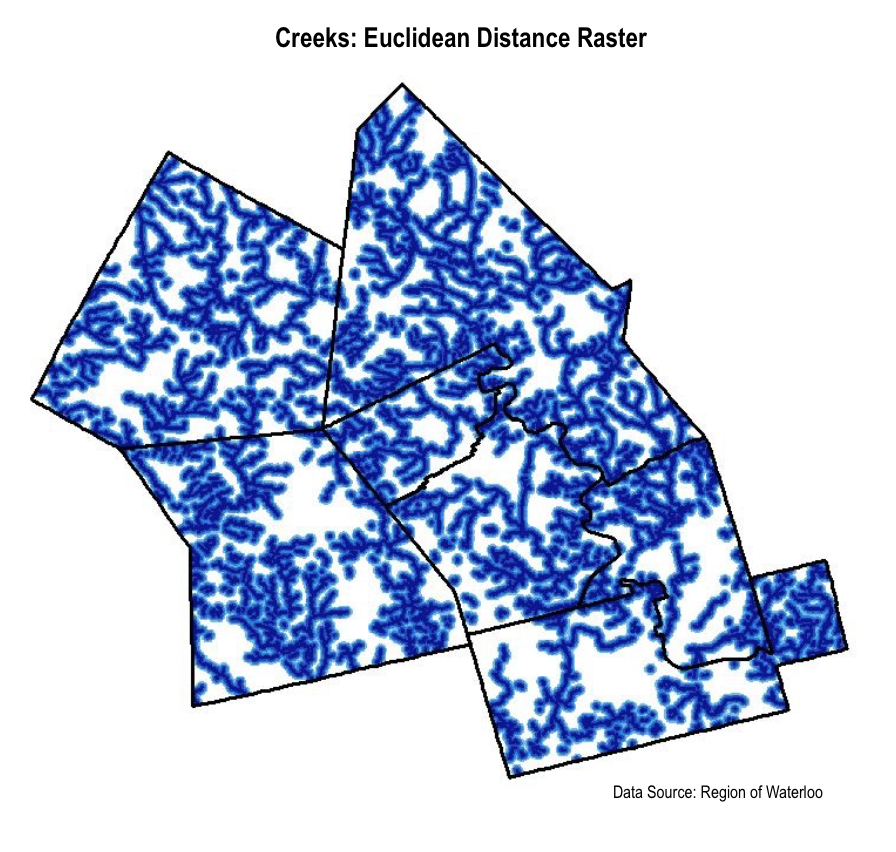
Also recognizing that our river layer only included major rivers, and that snapping turtles can hibernate even in small bodies of water, we realized the necessity of including a creek layer as well. From these two layers, we created Euclidean Distance rasters. We also created Euclidean Distance rasters with our road layer by separating roads into three categories: high use, medium use, and low use, and creating separate layers for each category. Using these new layers, we created Euclidean Distance rasters to symbolize the distance from different types of roads.

3. DETERMINING WEIGHTS for the MULTICRITERIA EVALUATION (MCE)

We then used an analytical hierarchy process (123AHP.com) to rank the importance of each factor for habitat suitability. We did this process twice – once for hibernation habitat, and again for nesting habitat. These values were added to our habitat suitability tables.

Hibernation Habitat Factor Weights:

• Distance to creeks = 0.25
• Distance to rivers = 0.21
• Land cover = 0.16
• Distance to high use roads = 0.15
• Distance to medium use roads = 0.13
• Distance to low use roads = 0.10

Nesting Habitat Factor Weights

• Soil type = 0.28
• Aspect = 0.15
• Land cover = 0.13
• Distance to high use roads = 0.12
• Distance to medium use roads = 0.10
• Distance to low use roads = 0.06
• Distance to creeks = 0.03
• Distance to rivers = 0.03

4. RECLASSIFICATION

We then reclassified all of our layers so that they would each have 5 classes, ranked from 1 – 5. A suitability score of 5 would be the most suitable. It was essential to have every layer classified in the same key (i.e. all had to be 1-5)!

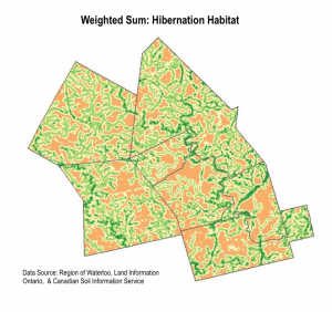
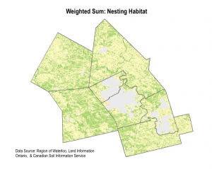
5. WEIGHTED SUM

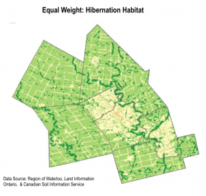
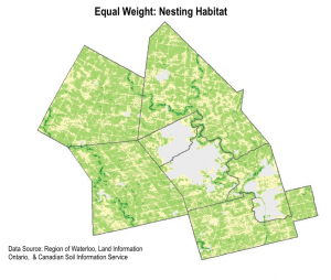
We used the weighted sum tool to determine the areas with highest habitat suitability. Essentially, the tool multiplies the suitability score by the layer weight for each pixel area.The output is a raster, where the highest pixel sums are the areas most suitable for snapping turtle habitat. We completed two weighted sum maps, for each hibernation habitat and nesting habitat. We also completed a sensitivity analysis by redoing the weighted sum with equal weights for each layer.

6. IDENTIFYING HABITAT PATCHES

The high level of detail in the weighted sum suitability maps made it difficult to detect real habitat patches. We decided to approach the display of data slightly differently by identifying coarser regions of priority habitat.

To do this, we conducted a fishnet analysis. First we created a 1000 cell by 1000 cell fishnet grid over the project area (each cell has a length of 15 meters) and converted our MCE results into points. We selected all points having a suitability score of 4 or higher, created a new layer with this selection, and joined it to the grid using the 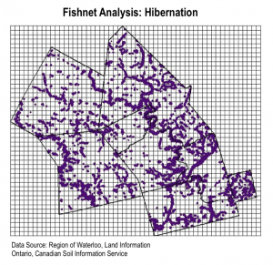intersect tool using sum as the merge rule. We did this twice – once for the hibernation habitat and again for nesting habitat. Once we had these two grid layers, we intersected these two layers with a sum merge rule. The resulting layer was a grid that displayed the areas with the highest sum of nesting and hibernation suitability.

The final step to prepare for analysis was to create a new layer that included only high use roads. We could then compare this layer to the highest suitability grid cells to determine where snapping turtle conservation interventions should be prioritized.