PRELIMINARIES 

This is the first of a series of blog posts I’ll be writing, detailing the work I’ll be doing with Dr. Catherine Neish on the subject of characterizing and comparing the surface roughness of terrestrial lava flows at Craters of the Moon National Monument with that of lunar impact melt flows.

There are 4 primary components to the problem: radar, LIDAR, surface roughness, and volcanics.

I began by getting up to speed on the background and literature of the problem . The obvious starting point was Catherine’s recent paper “Terrestrial Analogues for Lunar Impact Melt Flows” (Neish. et. al. 2017), for which my notes follow:

-Lunar impact melt deposits (LIMD) have amongst the highest observed radar returns at S-band, implying that rocks are on the order of this in size dimension
-ROUGH at the dm scale (S-band), but SMOOTH at metre (large) scales
-The morphology of LIMD correlates to their formation (ie. Emplacement conditions)
-Calculate roughness properties of terrestrial lava flows: RMS height, RMS slope, and Hurst exponent of the flows at a range of scales, via a ultra-high resolution backpack LIDAR system
-Compares these roughness properties with L-band radar (24cm)
-Compare all these roughness properties with LIMD properties from S-band (12.6cm), DTMs from NAC (Narrow-angle Camera) images, and surface roughness properties derived from LRO (Lunar Reconnaissance Orbiter) Diviner Radiometer measurements
-Lunar analogue is the LIMF from a lunar crater on the rim of Korolev X
-Explanations provided for the fact that radar returns of terrestrial lava flows differ from those of LIMF’s:
a) Different instrument calibration / methods
-ie. The specific way in which terrestrial radar data was downsampled, in order to better resemble its lunar counterpart
b) Fundamental differences in emplacement/cooling conditions on Moon
-For instance, the lunar erosional environment is primarily altered via impact gardening (when impacts stir the outermost crust of bodies without atmospheres), and fluvial/aeolian processes are not present like on Earth
c) Fundamental differences in the surface texture themselves (between lunar impact melt flows and terrestrial lava flows)
-ie. Since the lunar flows are of higher temperatures (due to superheating during impact), the lower viscosity of the melt could result in the melt travelling longer distances, cooling more slowly, and thus resulting in different surface textures (ie. smaller grain size?)
-Convective atmospheric cooling should also be different in a vacuum

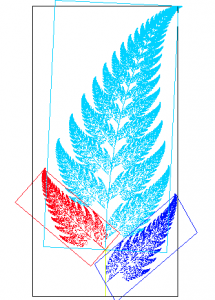
For brevity, other articles/posters/videos I perused include “Mapping Fresh Lava Flows with Multi-Wavelength AIRSAR and RADARSAT-2 Radar Imagery: Support of FINESSE Planetary Analog Missions” (presentation by Zanetti, Neish, and SSERVI FINESSE Team), which shows that using only 1 radar wavelength is insufficient to characterize a surface, owing from large observed discrepancies in CPR (Circular Polarization Ratio), some introductory chapters  of “Volcanism of the Eastern Snake River Plain, Idaho: A Comparative Planetary Geology Guidebook” (NASA 1977) to get up to speed on the geology & volcanology of the area of interest; a very hip, lucid primer on fractals (“Fractals are typically not self-similar” (see example of a completely self-similar fractal below), from which I learned that fractals are defined as shapes with non-integer dimension, or alternatively, as shapes that are rough, and stay rough regardless of scale; “Lava Flow Surface Roughness and Depolarized Radar Scattering” (Campbell and Shepard 1996); “The Roughness of Natural Terrain: A Planetary and Remote Sensing Perspective” (Shepard et. al. 2001), which provides a very organized lay-of-the-land in standardizing the parameters used to measure surface roughness, allowing for the meaningful  comparison of roughness determined by different instruments/methods; “Roughness of Hawaiian Volcanic Terrains” (Morris et. al. 2009), which implements a 2D surface roughness measure (ie. the 2D analogues of the 1D RMS height / RMS slope / Hurst exponent), as opposed to the paradigm of taking 1D roughness profiles; and “Allan Variance computed in Space Domain: Application to InSAR data to characterize noise and geophysical signal” (Cavalie and Vernotte 2016), which determined expressions for the transfer functions of a 2D spatial Allan variance (both Cartesian and polar). Regarding that last one, I am unfortunately at a loss as to how those transfer functions are actually applied in order to calculate the Allan variance.

MINI-PROJECT 1: NUMERICAL COMPUTATION OF ROUGHNESS PARAMETERS 

One component of this project involves the methodology of actually calculating the roughness parameters espoused by Shepard et. al. (2001). To that end, Catherine gave me a script to play around with in IDL (a software package / programming language geared towards image processing applications). I have been attempting to ‘translate’ the script to MATLAB – but have had difficult in obtaining the same values for Ina Caldera as Catherine had in her 2017 paper. For reference, here’s what Ina Caldera actually looks like (as a mosaic):

The idea is then that the elevation at each point can be calculated, by essentially taking a low-pass filter of heights of the surrounding points, then fitting a line to this collection of points. This ‘large-scale trend’ can therefore be subtracted from each point, allowing us to look in at the small-scale roughness that we’re really interested in.

This process can then be repeated, but by increasing the spacing between the points and calculating the Allan variance (essentially the difference between 2 consecutive points), then plotting the Allan variance against the point-spacing size in log-log space, in order to come up with what’s called a ‘variogram’.

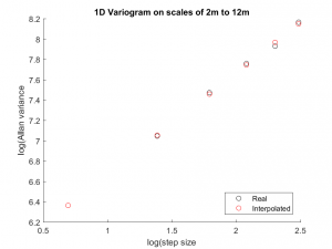
This variogram is really nifty: the slope is the Hurst exponent, which is related to the fractal dimension (ie. how the roughness of the surface changes at different scales), while the y-intercept of the graph is the RMS slope, which is another measure used to characterize a surface’s roughness (specifically, the deviation in space of the surface’s slope). Ultimately, this allows us to come up with plots like the following, for Hurst exponent and RMS slope, respectively.

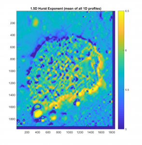
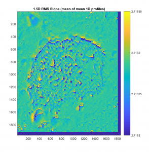
I was happy to see that the plots roughly resembled the picture! And then crestfallen to discover that the actual magnitudes of the numbers don’t really make sense. This is ongoing, but I believe that the devil is in the details: during the script ‘translation’ from IDL to MATLAB, quite a few things changed which I had initially been unaware of! I made a list of the differences I’ve encountered, for reference:

Comparing MATLAB and IDL

MATLAB

IDL

a) Indexes start at 1 b) Arrays are ordered [row , column] c) Does not automatically round numbers d) Polynomial fitting function (polyfit) has coefficients ordered in descending powers e) [1:5:11] indicates a matrix starting at 1, incrementing by 5, and ending at 11 f) Arrays are automatically in floating point format, in either single or double precision (default is latter) g) Array elements are accessed with round brackets () h) To access all array elements, use : (eg. A(1,:) ) i) Use back-slashes when specifying file paths j) Semi-colon suppresses output k) For loops have format: for dn = [dni:1:dnf] …… End l) Scripts (though not have functions) don’t have any special formatting requirements

a) Indexes start at 0 b) Arrays are ordered [column , row] c) Automatically rounds numbers down.. d) Polynomial fitting function (poly_fit) has coefficients ordered in ascending powers e) [1:11:5] indicates a matrix starting at 1, ending at 11, and incrementing by 5 f) Floating point format must be specified in arrays (using fltarr) g) Array elements are accessed with square brackets [] h) To access all array elements, use * (eg. A(1,*) ) i) Use forward-slashes when specifying paths j) Semi-colon used for commenting k) For loops have format: for dn = dni, dnf, 1 do begin …… Endfor   l) Scripts (procedures, abb. as pro) have format requirements: pro script_name …… end -Calling procedures (dark blue): name,arg1,arg2,… -Calling functions (ultramarine blue): fltarr(arg1,arg2)…

 

Hopefully, by accounting for these differences, I’ll be able to get accurate results in the future. I’ve also been thinking about how to extend the idea of measuring surface roughness to 2 dimensions, which would allow for a more realistic comparison with radar remote sensing data, which is sensitive to the full 3-dimensional topography of a surface. A basic calculation however, shows that the approach I’m thinking about (which I may describe in a future post) would require 400 days of computation time…!