Just kidding – time isn’t a consideration in our research. Yet. For now, we’ll stick with 3 spatial dimensions.

And so our adventures in the wondrous world of surface roughness continue!

As illustrated in my last post, during which I showed some maps of the calculated roughness of Ina D Caldera on the Moon, the traditional way to pre-process the topography maps of surfaces and calculating their roughness parameters is to perform ‘de-trending’ for every 1-dimensional profile. In other words, the best-fitting linear trend along a profile (each of which has a length of 100m, in our case) is subtracted, resulting in a de-trended profile, for which roughness parameters such as the RMS Slope and the Hurst exponent are calculated. The process is then repeated for every point in the 2-dimensional array of heights that constitutes the digital elevation map (DEM) of Ina D Caldera.

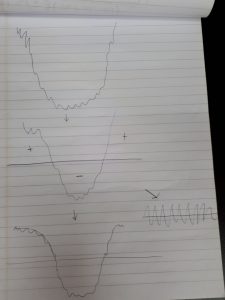
I see there being 2 problems associated with this methodology, however. The first is that this is an inherently local procedure. What this entails is that the topography of the de-trended points changes with respect to each different profile position, and by extension the roughness parameters that are calculated based on these de-trended heights will also change. The second is that I am not convinced that the linear de-trending is actually removing topography (where I define ‘topography’ as the large-scale variation in the height of a surface). Indeed, conversely, it could be artificially enhancing roughness in areas with very little of such. For instance, imagine a surface that is, to first approximation, symmetrically U-shaped (see below, top plot), with finer, ‘rough’ detail inscribed upon it.  (Note that the scale is vertically exaggerated – the same principles should apply nonetheless.) Since, to first approximation, the linear trend is flat and about 0 (middle plot), the ‘de-trended’ profile would be identical to the raw profile (bottom-left plot)! Rather, the desired plot would be more of the form of the bottom-right plot: depicting only the small-scale deviations from the overall, large-scale U-shaped topography.

 

It turns out that this is not a new problem; indeed, extensive methods have been devised in the discipline of surface metrology (a subdivision of mechanical engineering) to deal with the division of surfaces into the surface roughness we’re actually interested in and the large-scale topography in which we are not (typically ‘micro-topography’ in metrology, seeing as the field largely deals with machined surfaces on the scale of millimetres, micrometres, and even nanometres (for the study of atomic ‘surfaces’)). In the metrology vernacular, these small-scale and large-scale components are termed ‘roughness’ and ‘waviness’, respectively, where the roughness profile is simply the primary profile (raw data) subtracted by the waviness profile. The devil is however in the details: how do we determine where the barrier lies between roughness and waviness? Should this be a sharp threshold (eg. all surface height variations at scales of <1m are part of the roughness profile and all those at scales of >1m are part of the waviness profile)? Or should there be a continuum; a more gradual transition?

Enter the Gaussian filter, which is of the latter variety. In its 1D implementation, its ‘transfer function’, which defines how much surface ‘signal’ gets transmitted as a function of the spatial wavelength, it forms a relatively smooth distribution. We define a ‘cut-off wavelength’ at which exactly 50% of the signal gets transmitted (1mm in the test case below). Specifically, we use a high-pass filter, which entails that wavelengths above this cut-off get more and more attenuated, while wavelengths below are more and more intact.

The thing is – how we define our cut-off wavelength ultimately boils down to scale. On the Moon, where we lack a priori knowledge, who is to say that a 5m feature constitutes roughness, or that a 10m one, or a 20m does? I read an interesting review paper (“Roughness in the Earth Sciences” (Smith 2014)), essentially states that there does not exist across the earth sciences a standard definition of roughness. Surface roughness plays a large role in disciplines ranging from hydrology and oceanography to geomorphology, glaciology, and myriad other fields, yet the ‘roughness’ that’s being talked about is almost always arbitrarily defined, seeing as the ‘waviness’ (ie. large-scale topography) is not typically specified. This often makes it difficult (or to be cynical, meaningless) to compare measures of roughness even within the same discipline – much less across disciplines!

But why restrict ourselves to 1 dimension at a time? After all, we do possess a 2-dimensional grid of heights, and can take advantage of the additional spatial information therein. The principle behind the 2D Gaussian Filter is relatively straightforward:

i) Take the 2D Discrete Fourier Transform (2dDFT) of the 2D grid of heights, then the 2dDFT of the Gaussian weighting function, where the 2dDFT is

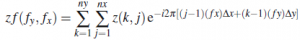
where z(k,j) is the 2D grid in question,

f_x is the spatial frequency in the x direction,

f_y is the spatial frequency in the y direction,

nx is the number of grid cells in the x direction,

ny is the number of grid cells in the x direction,

dx is the sampling interval in the x direction,

dy is the sampling interval in the y direction,

 

ii) Take the 2dDFT, but this time for the Gaussian weighting function (a smooth pulse, shown below)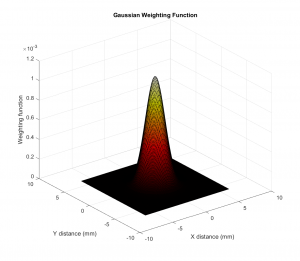 

which is defined by the equation

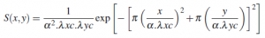
(essentially just two 1D Gaussian functions (one of each in the x/y directions) multiplied together)

where lambda*x*c is the cut-off wavelength in the x direction, and lambda*x*c is that in the y direction

 

iii) Multiply these 2 together Fourier-transformed functions together

iv) Convert back to the spatial domain by taking the inverse Fourier Transform (2dIDFT) of this product

 

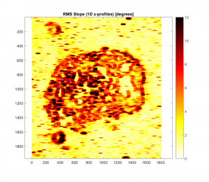
Having explained in long-winded fashion what this filter’s all about, here’s the result of applying the 2D Gaussian filter to the Ina D Caldera DEM, for RMS slope.

-Here’s the RMS Slope map (in degrees), with a 9×9 median filter applied, but no filtering:

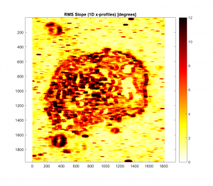
-And here’s a similar map, but with a 2D Gaussian filter applied with a cut-off wavelength of 100m:

-Cut-off wavelength of 200m:

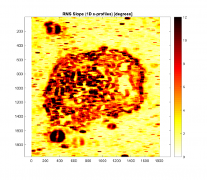
-Cut-off wavelength of 400m:

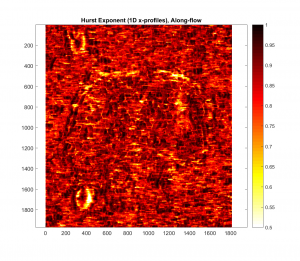
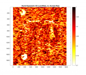
And the analogous plots for the Hurst exponent:

-9×9 median filter, no Gaussian filtering:

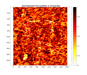
-Gaussian filter with cut-off wavelength of 100m:

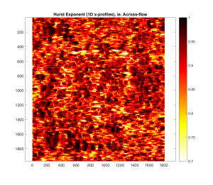
-Cut-off wavelength of 200m:

-Cut-off wavelength of 400m:

For both cases, it appears that as the Gaussian Filter’s cut-off wavelength is increased, the roughness parameter map in question more closely resembles the one with no Gaussian filter applied. This makes intuitive sense, because as the cut-off wavelength is increased, more and more of the spatial frequency signal is retained.

 

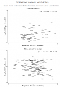
In other news, I made a serendipitous discovery: that roughness is also used in the social sciences, albeit given a different name – ruggedness. In “Ruggedness: The Blessing of Bad Geography in Africa” (Nunn and Puga 2012), it is shown how, albeit with a weak statistical correlation, higher surface roughness in African  nations is correlated with higher incomes. The explanation given? That it all has to do with history: from 1400 to 1900, rates of slavery were lower in countries with rougher surface, perhaps because such surfaces afforded protection to the peoples of these nations from colonizers. This historical iniquity is then attributed to present-day differences in economic growth amongst African Nations.

 

 

The ruggedness/roughness parameter in question is measured by a simple ‘nearest neighbour’ approach, in which the root-mean square deviation between each and every point adjacent to a central point (including diagonals) is summed, for every point on a DEM (see below).

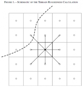
This is encapsulated in the formula

where r is the row number of the central pixel,

and c is the column number of the central pixel.