Now I’ll move on to some new, fully 2D roughness maps produced by revised roughness algorithms, that fully take into account potential directional bias (which is inherent to 1-dimensional profile methods). Again, we’re looking at our test DEM dataset of Ina D caldera on the Moon.

I: Ina D 2D Roughness Maps 

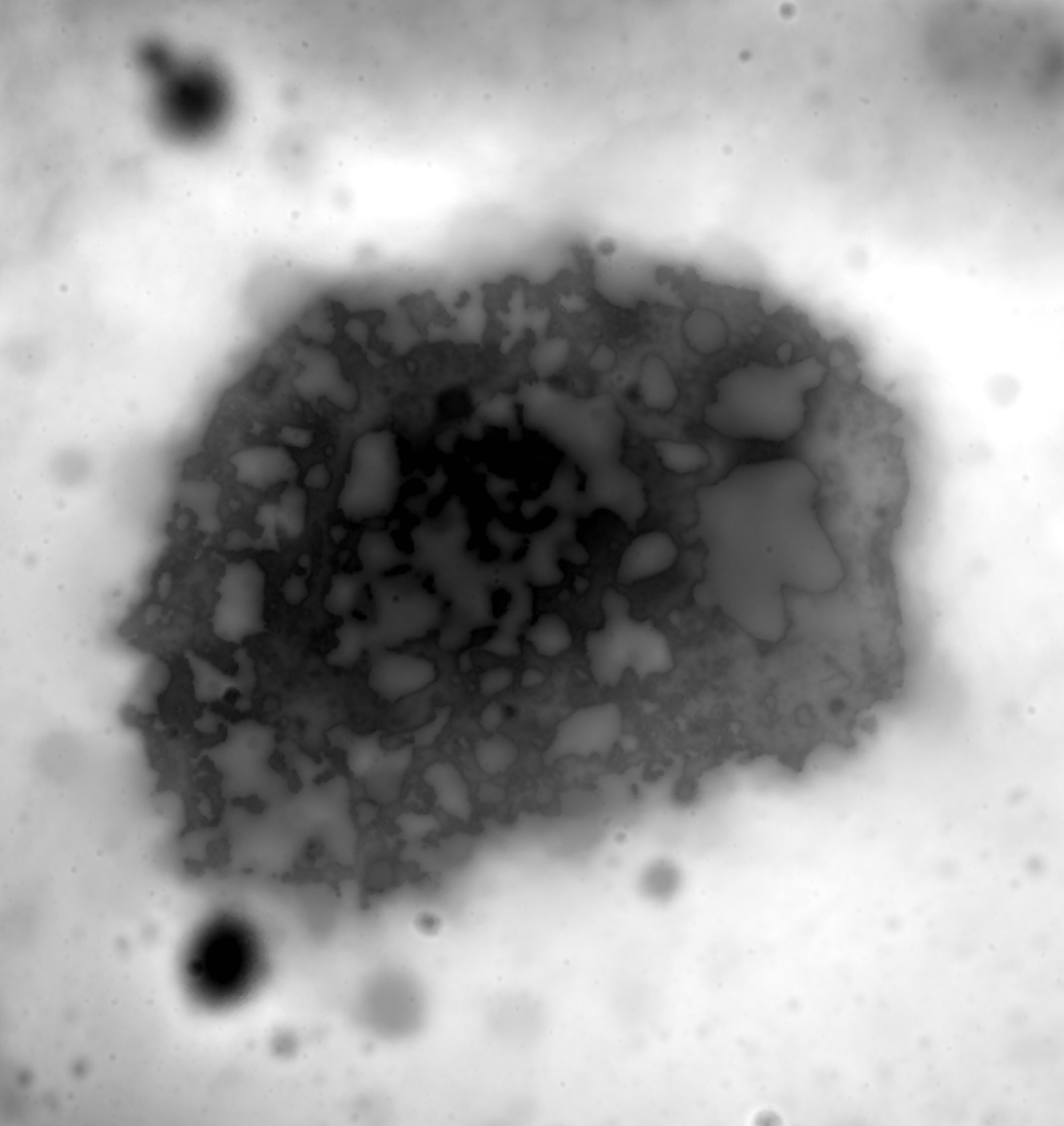
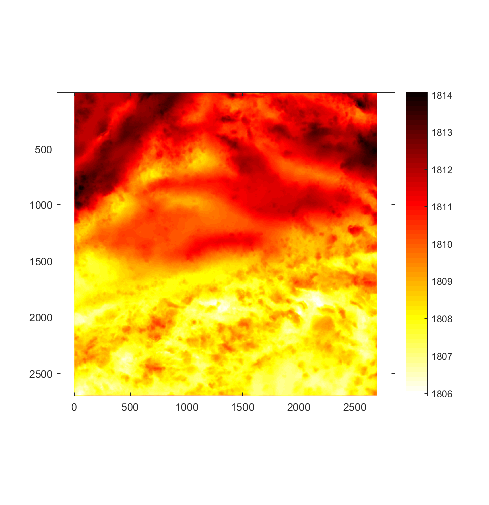
Here’s the reference DEM, with which we can see what features the roughness maps emphasize (or do not).

 

The RMS slope and Hurst exponent are calculated in 2 dimensions (or 3, if height is included) via the algorithm described in detail here. (This document is also useful for getting a handle on the terminology with which I describe the various parameters used in the roughness algorithm). Note that all of the following roughness maps were calculated using elevation data that was pre-processed via a 2D Gaussian filter with a cut-off wavelength (50% transmission threshold) of 100m (chosen to match the 10om profile length used to calculate the analogous 1D roughness parameters).

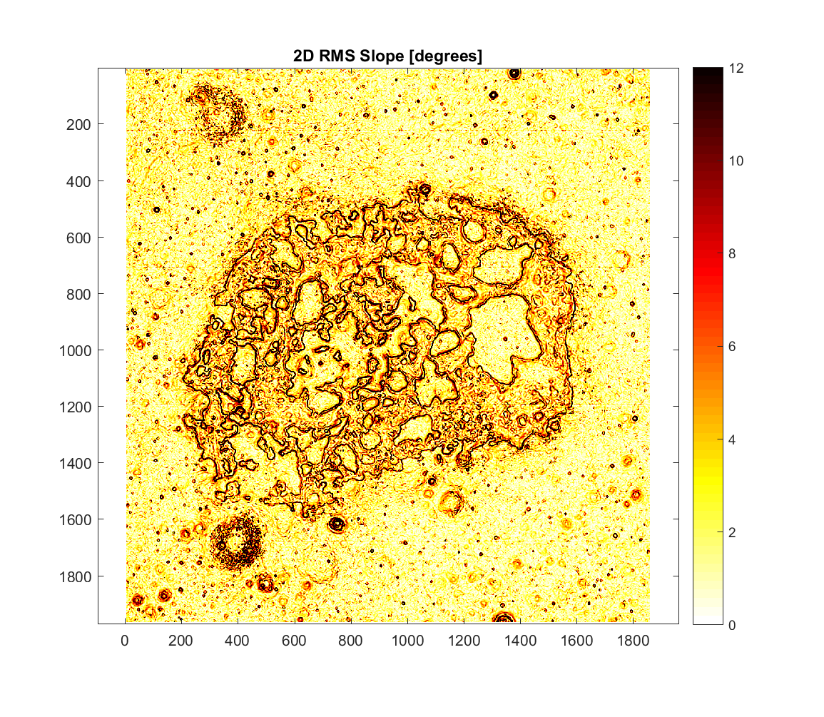
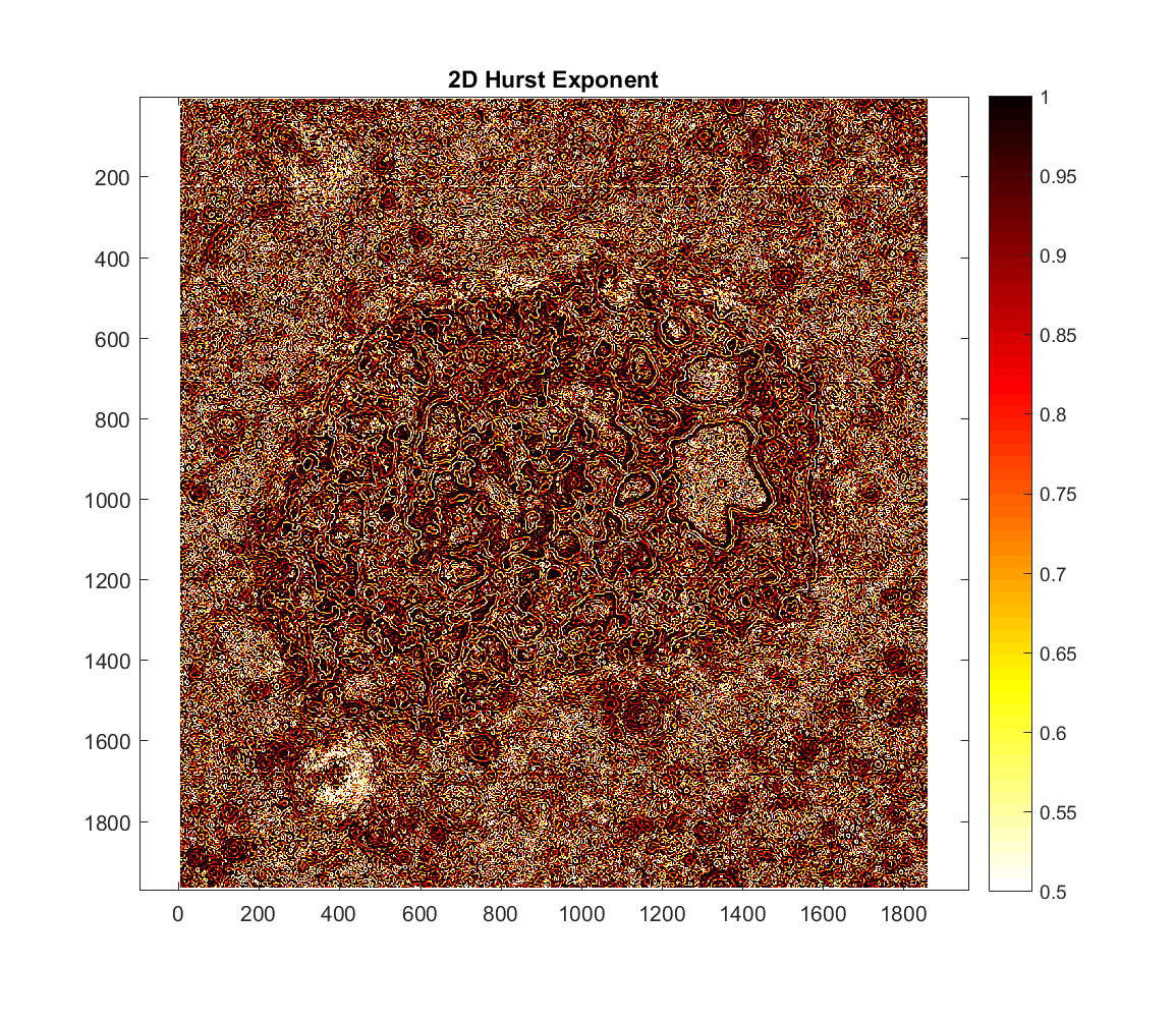
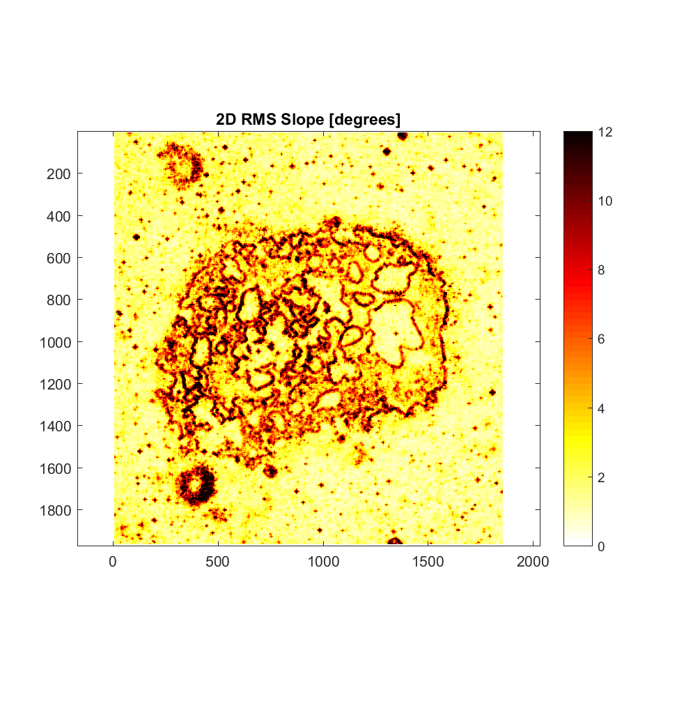
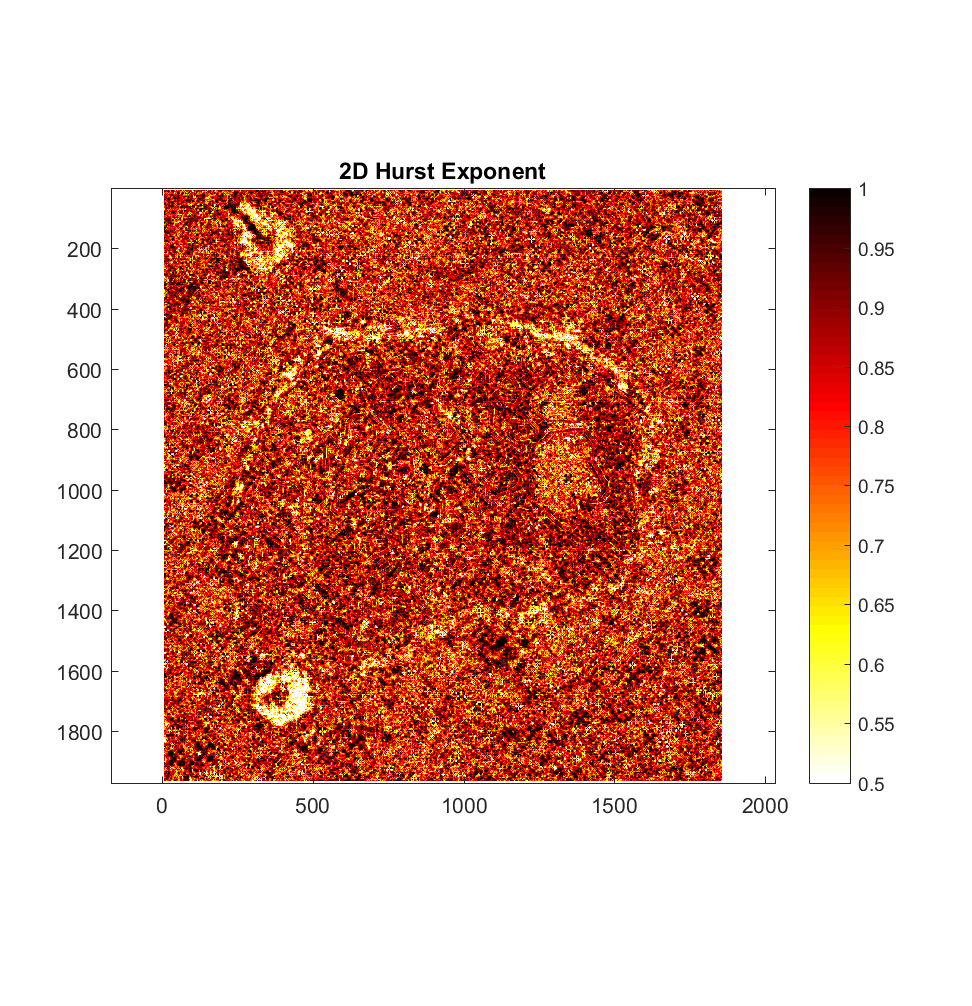
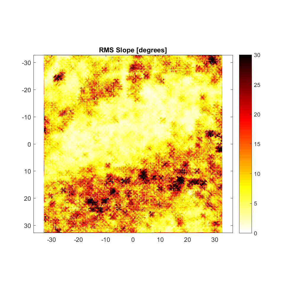
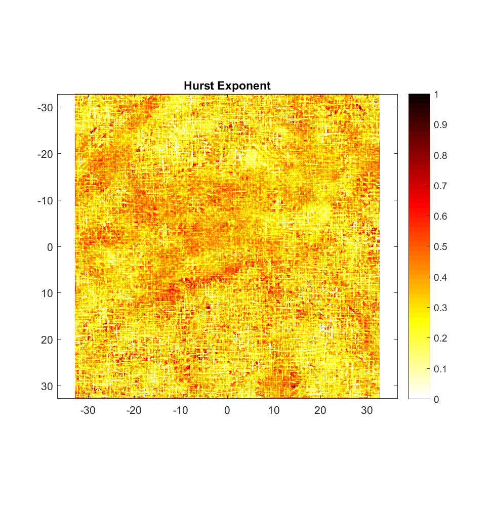
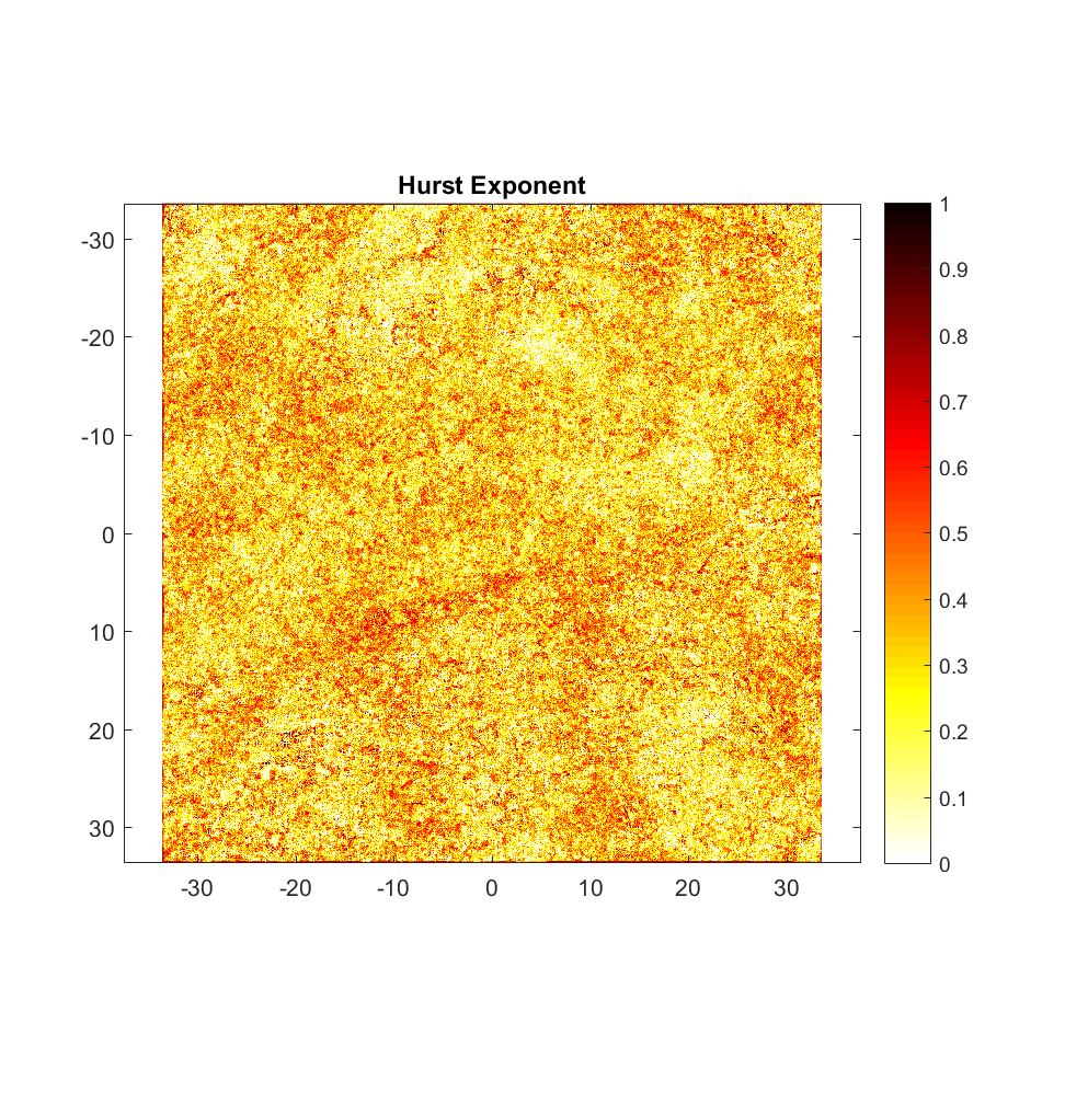
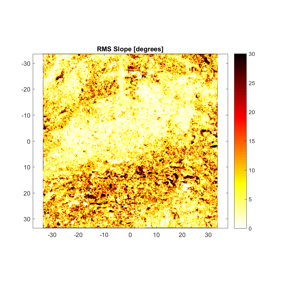
In the first case, only one pair of points in each direction is used to calculate the RMS Deviation for a particular step size. We see that the maps look fairly free of directional bias, in addition to being quite highly resolved. In particular, the 2D RMS Slope map shows the walls within the caldera quite well (the thin black lines surrounding regions). Meanwhile, the 2D Hurst Exponent map shows a marginally larger higher value inside the caldera than outside it, and also emphasizes caldera walls, which have H values approaching and even exceeding 1. While values of H>1 are unphysical, I hypothesize that the errors associated with these values are sufficiently large that the values may not in fact be >1. While I have also calculated accompanying maps of the errors associated with these parameters at each points, the error calculation methodology may not fully account for the substantial degree of uncertainty that accompanies calculation of the Hurst exponent.

8-connected, Gaussian-filtered roughness with 5×5 moving (local) cells: 

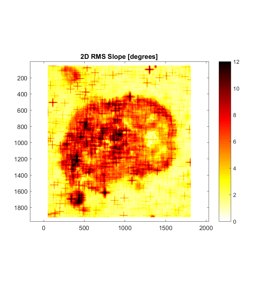
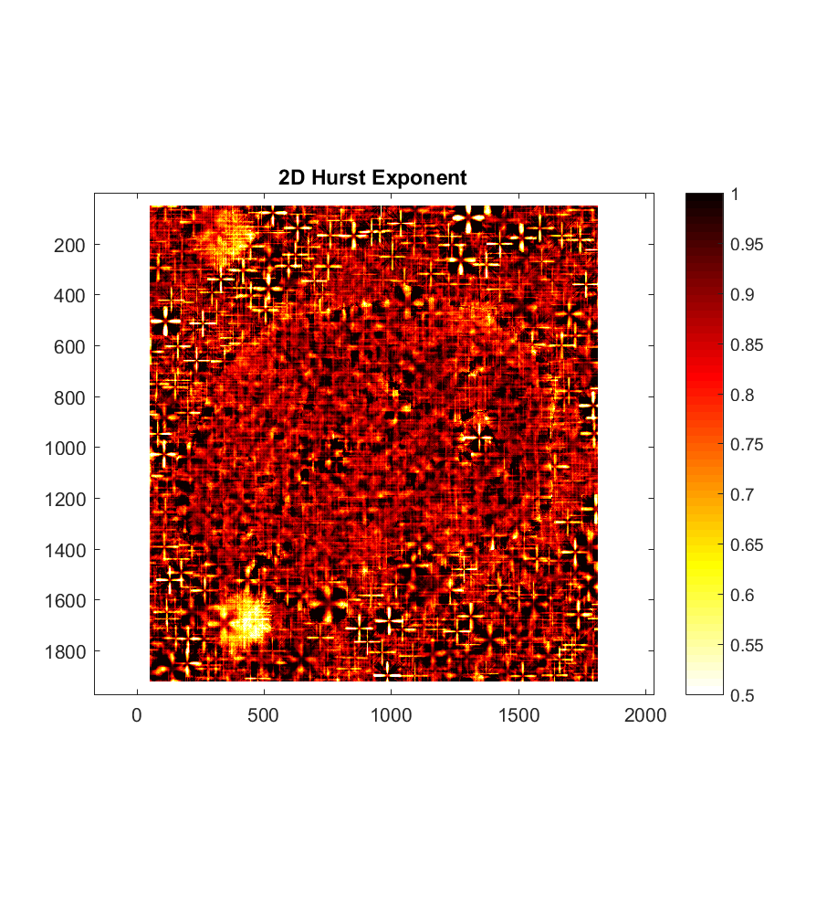
The next 2D roughness maps are analogous to those before, but with larger 2D ‘cell’ sizes (analogous to 1D profile lengths), such that multiple pairs of points are used to calculated the RMS Deviation for a particular step size. Disconcertingly, large, plus-sign shaped 2D ‘artifacts’ seem to be the result, for both roughness parameter maps. (See “II: Ina D 2D Roughness Artifacts” for an attempt to explain the nature of these artifacts).

8-connected, Gaussian-filtered roughness with 40×40 moving (local) cells: 

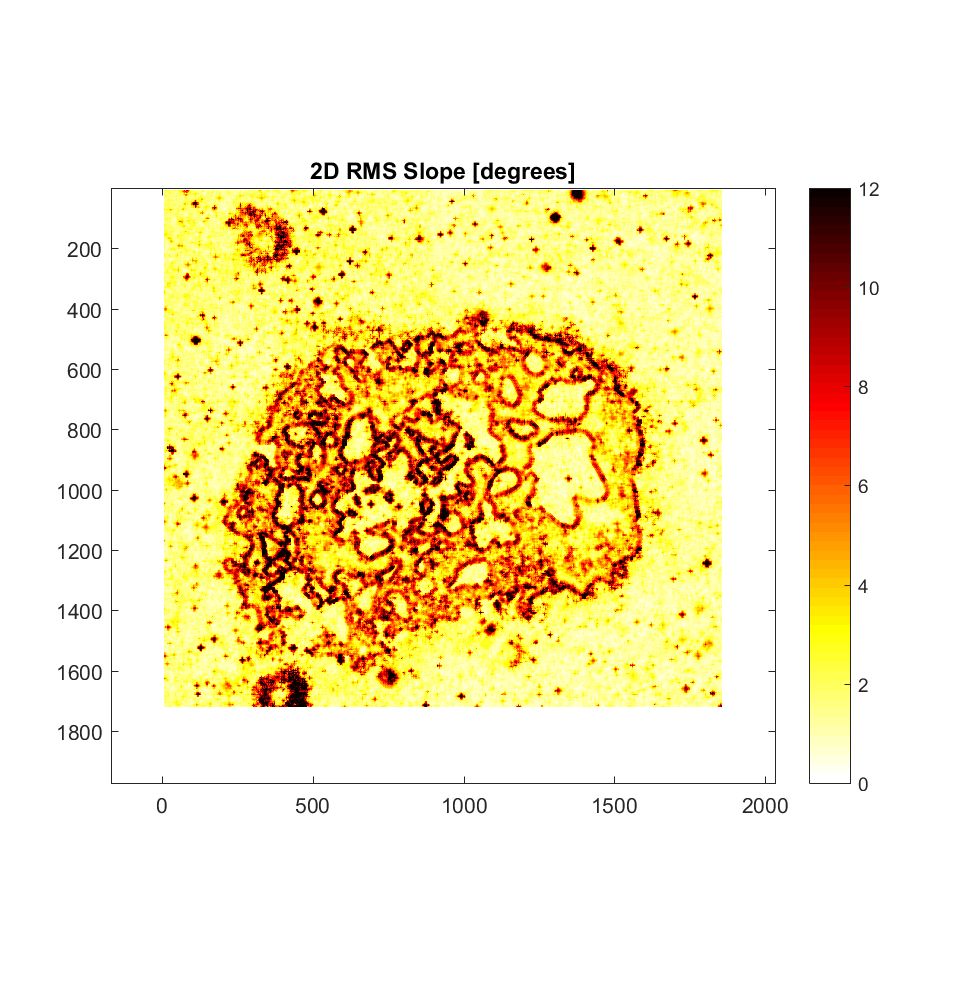
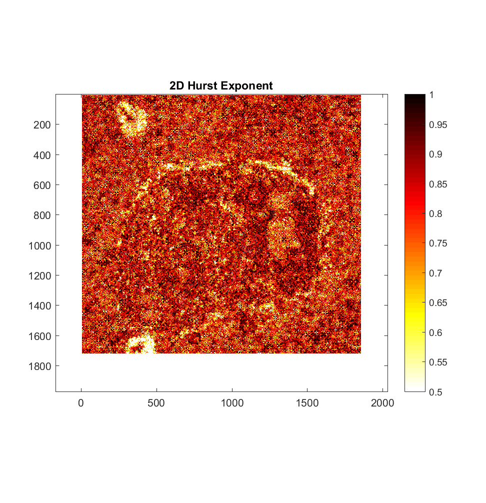
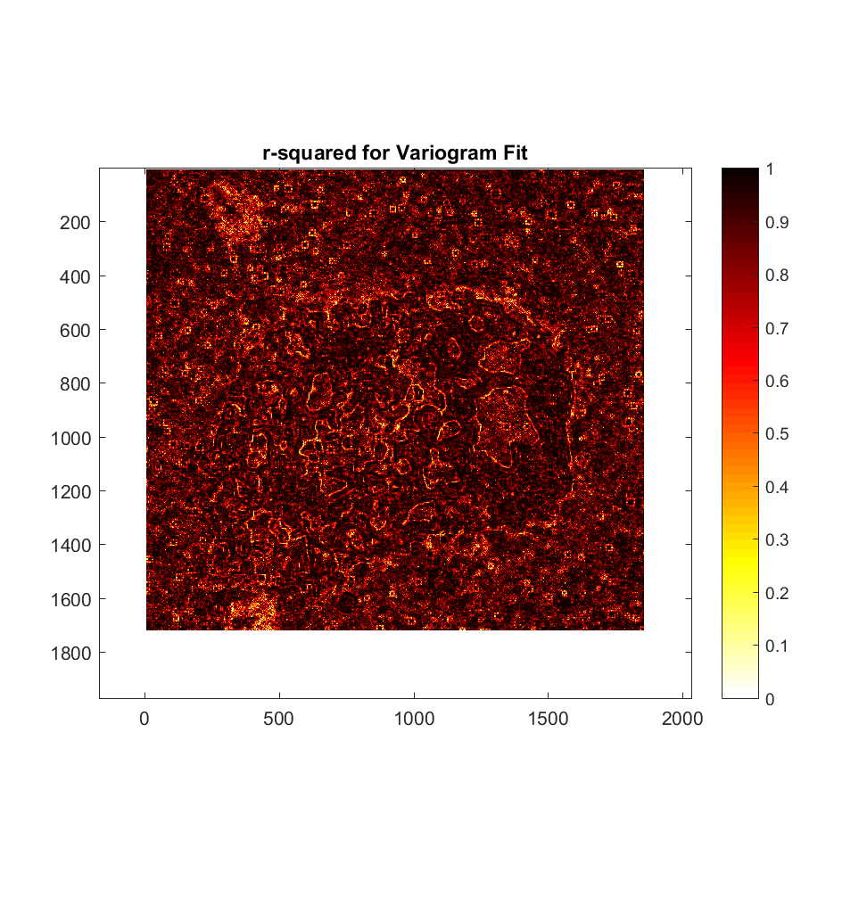
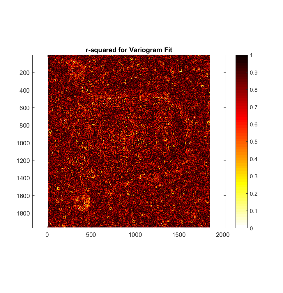
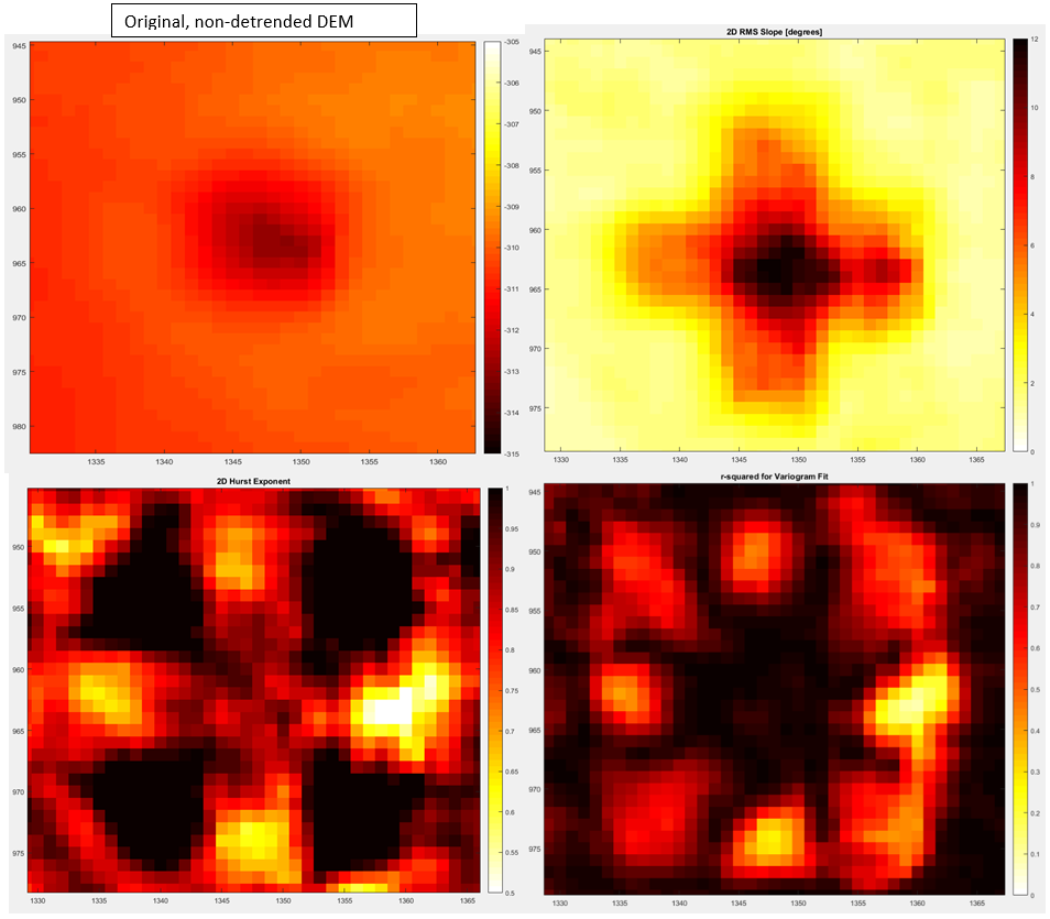
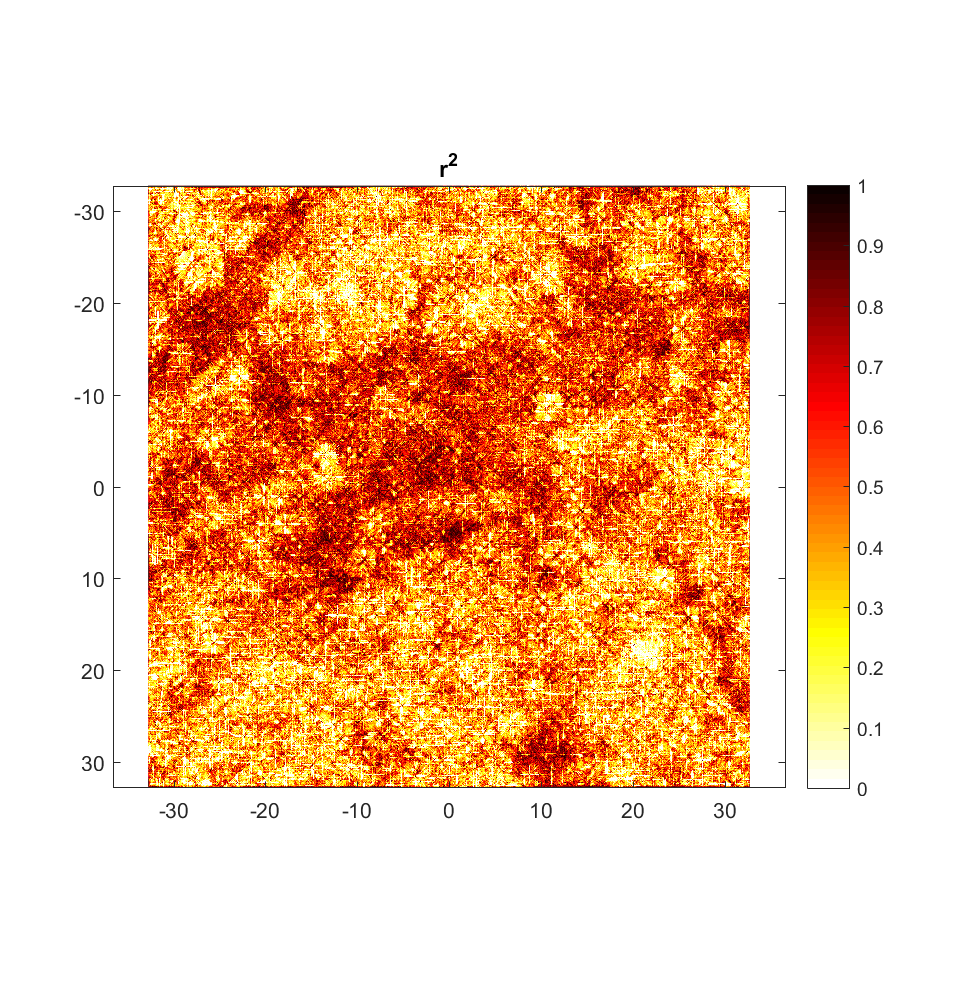
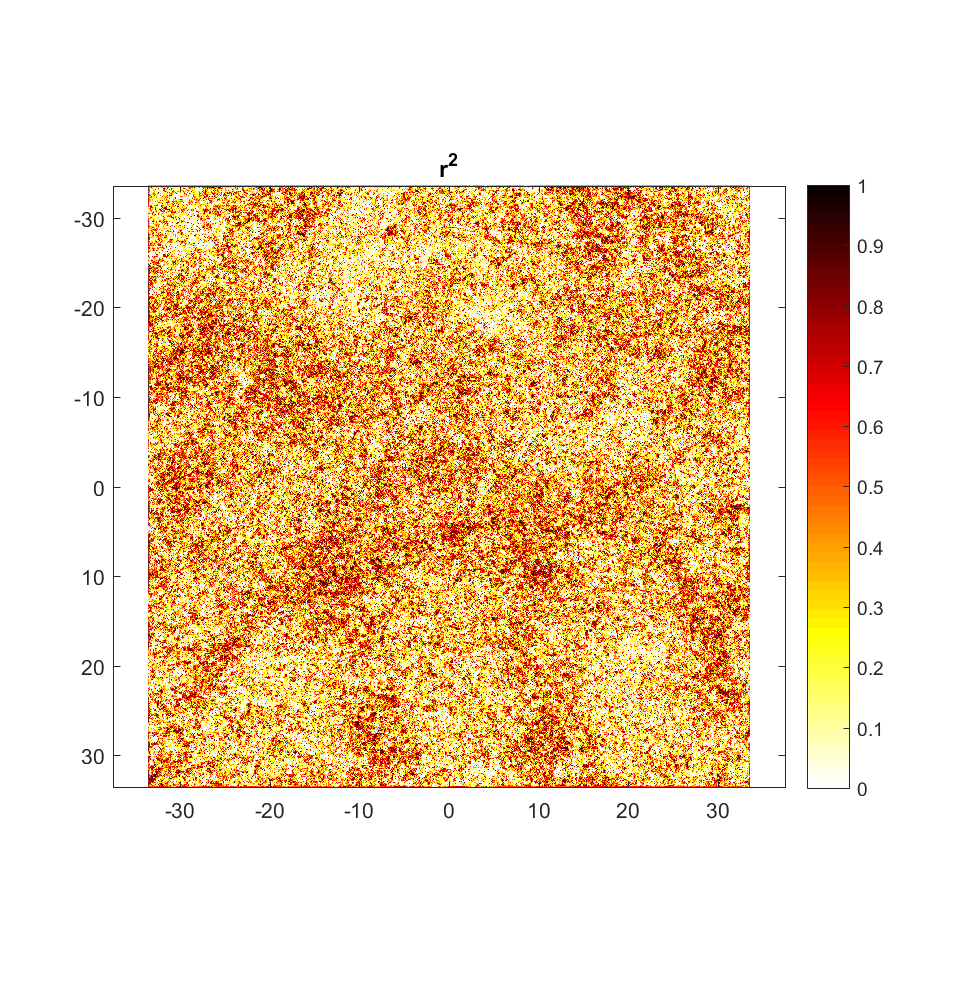
In an attempt to alleviate these artifacts, I reduced the (local) cell size. [I acknowledge that, strictly speaking,  such a decision goes against ‘Sheperd’s 10% Rule’ (from Sheperd et. al. 2001), in which it is stated that it is desirable to use profiles at least 10 times longer than the largest scale (ie. step-size) utilized on the variogram. However, given that this rule was conceived of in the interest of using an adequate number of samples to derive the points on the variogram in 1D, the larger number of samples inherently present in 2D owing to the higher dimensionality should entail that this rule can be relaxed.] The resulting roughness maps, as expected, more closely  now resemble the 5×5 cell maps, though upon closer examination, the strange ‘plus-sign’ shaped artifacts remain both for RMS Slope and Hurst Exponent. A map of r-squared was also calculated, showing the value of r^2 (the coefficient of determination) for the variogram at each point. Intuitively, this gives us a quantitative measure of how well the assumptions used to derive RMS Slope and the Hurst Exponent from our variograms actually holds up. Namely, we are assuming that log(RMS Deviation) scales linearly with log(step-size); as the plot shows, however, a significant number of the variograms/points have r^2 values less and even much less than 1. The r^2 values are lowest, upon comparison with the original mosaic DEM, at the caldera borders; this is to be expected, as the RMS Deviations calculated at such points will exhibit a high degree of anisotropy, the slope varying extensively with respect to direction.

8-connected, Gaussian-filtered roughness with 17×17 moving (local) cells: 

 

 

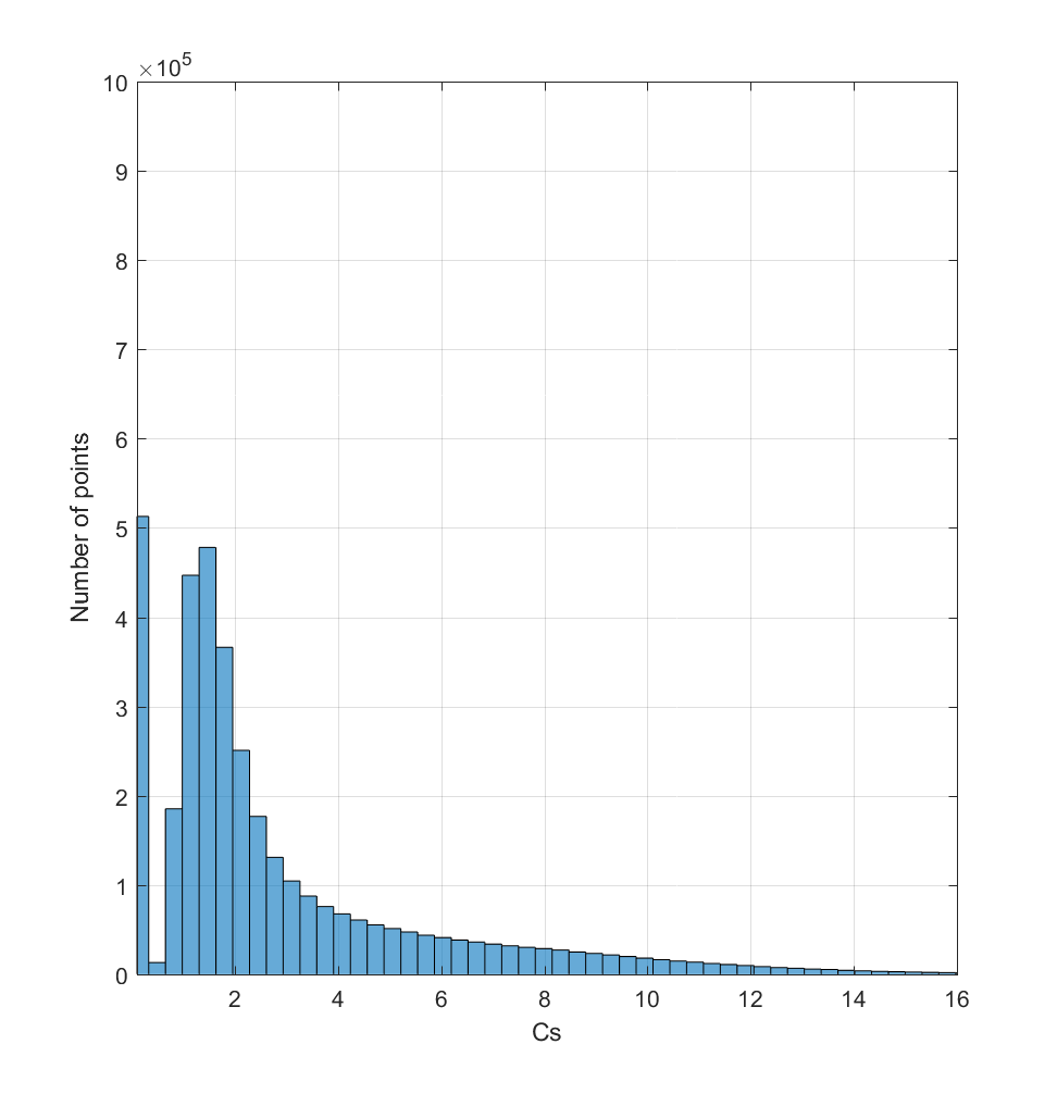
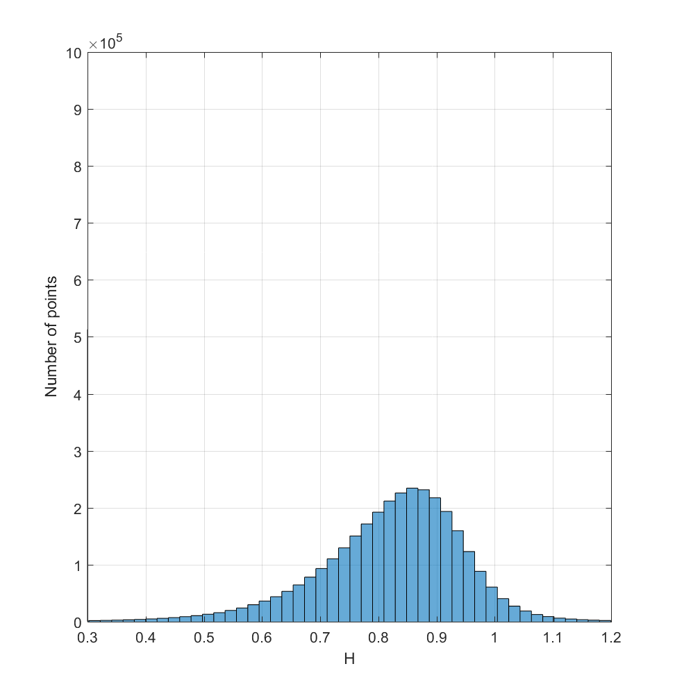
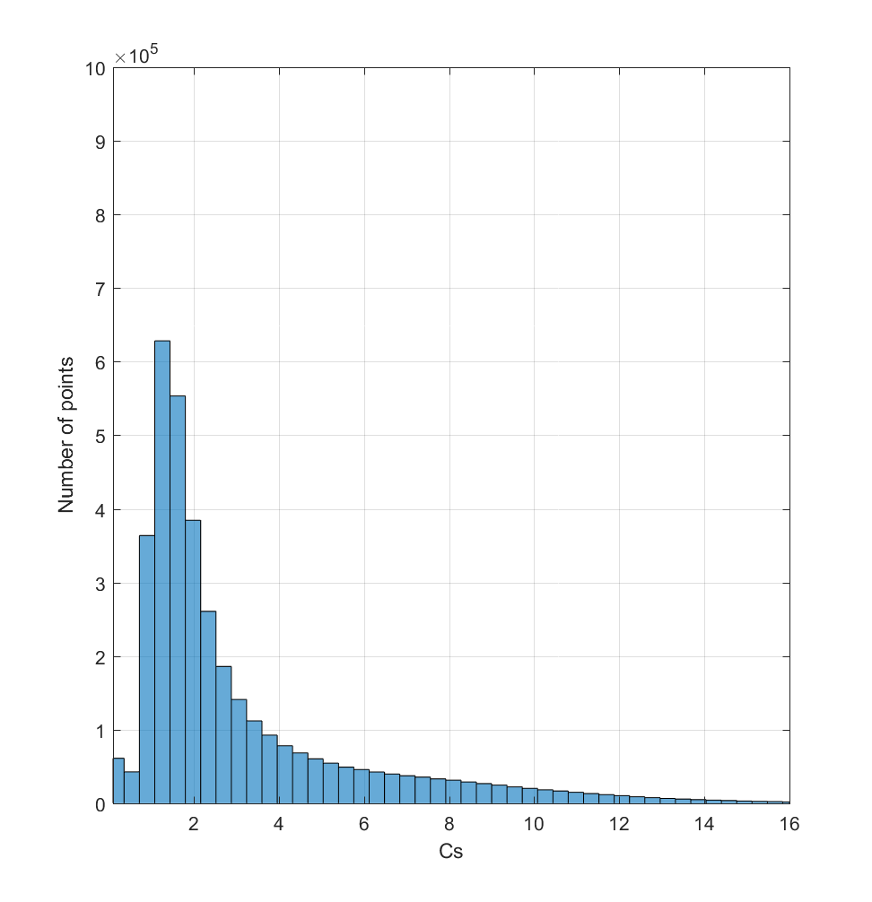
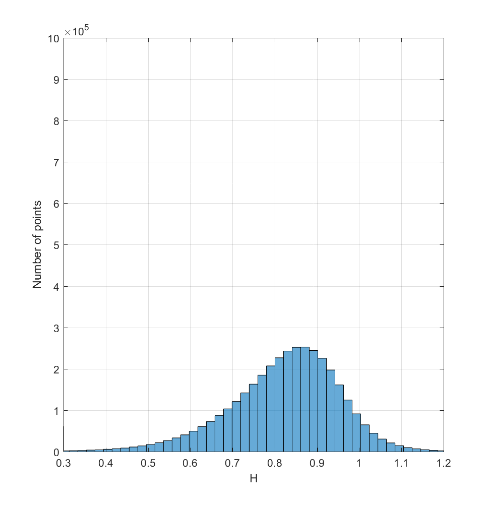
Next, histograms of the distribution of RMS Slope (Cs, in degrees) and Hurst Exponent (H) values at each point imply that Cs has a rough power-law distribution, peaking at ~2 degrees and declining rapidly in abundance for steeper values. (NB: The spike at 0 is irrelevant, being the value of the white space surrounding the map), while the H distribution peaks at the relatively high value of ~0.85, with the majority of values concentrated between 0.6-1.

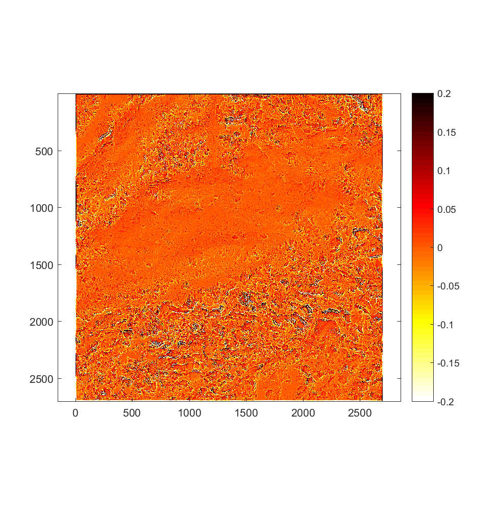
Next, I tested how the effect of changing the pre-processing method employed; namely, the method to detrend the elevation data.

 

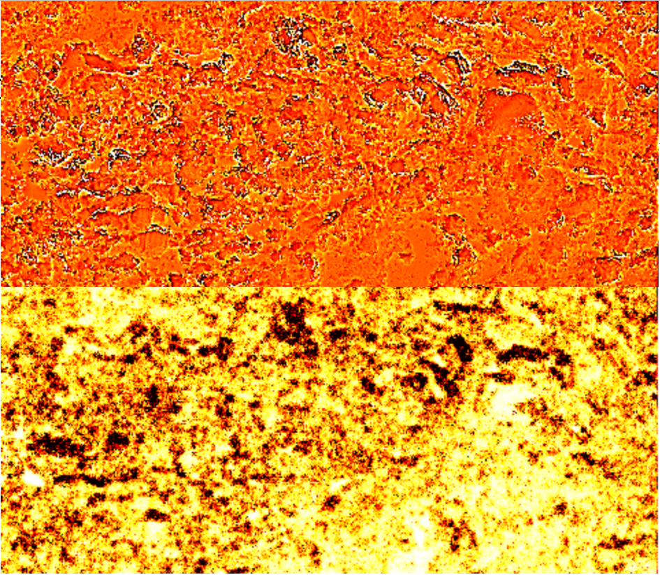
Analogous plots, for planar detrending (ie. fitting a plane via least-squares optimization) over a 17×17 local cell.

 

 

 

 

 

 

 

 

 

 

 

II: Ina D 2D Roughness Artifacts 

Artifacts: attempt to see why we see strange ‘plus-signs’, ‘crosses’, and other artificial-looking structures in our roughness maps…

 

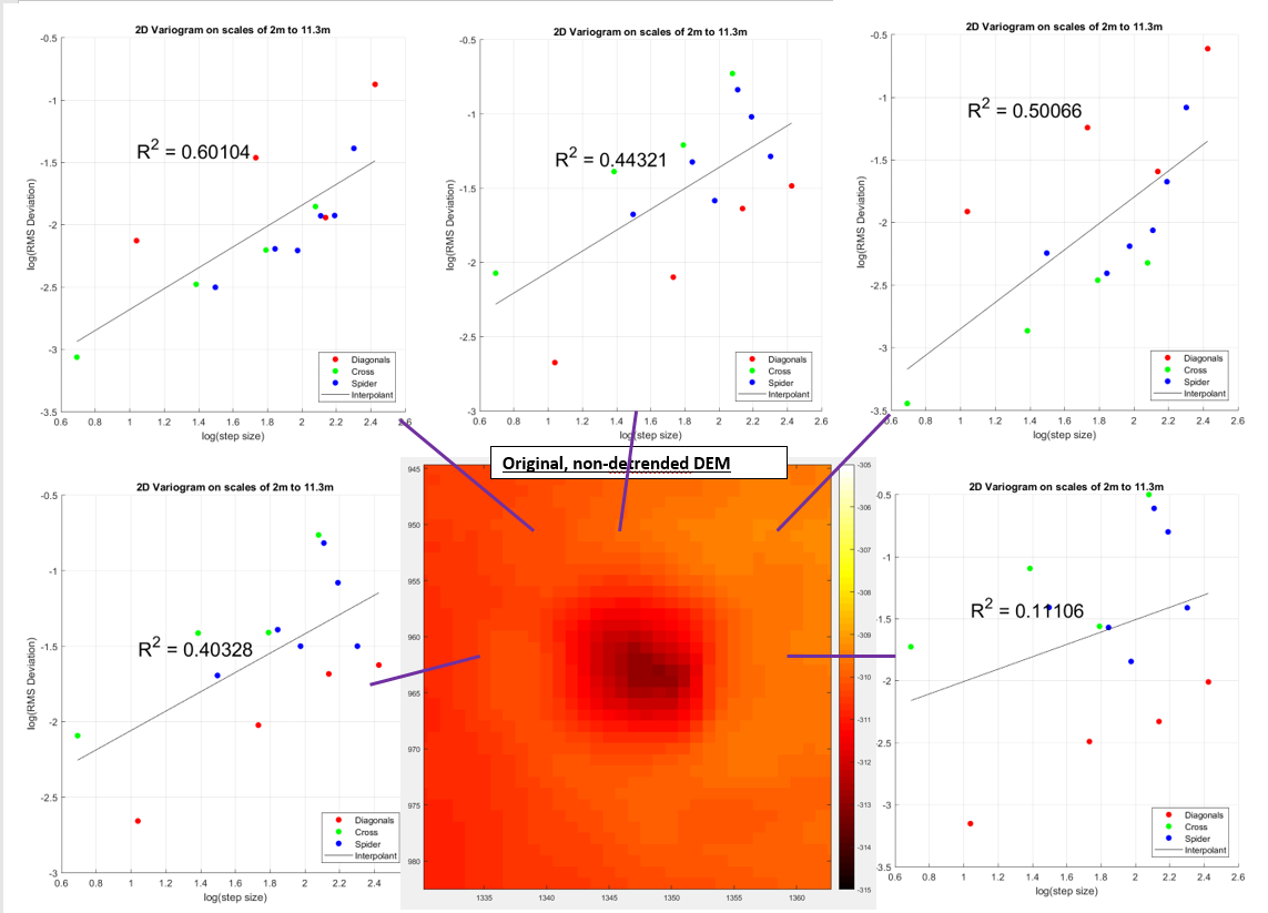
-Variograms surrounding central depression show anisotropic RMS Deviation, RMS Slope, and Hurst Exponent

 

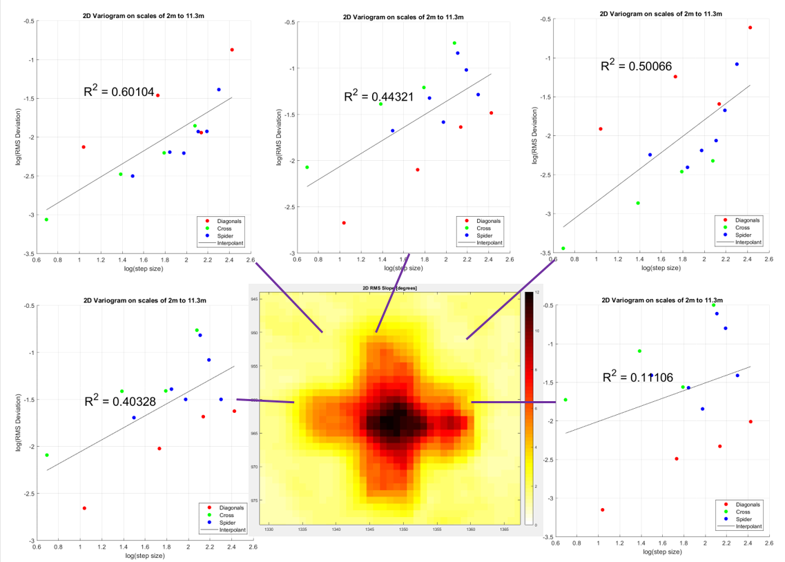
-‘Plus-sign’ shape can be explained by high cross-arm values in addition to moderately high spider-arm values in orthogonal directions away from the central depression

-Conversely, for corner variograms, only one diagonal-arm will reach the central depression, resulting in low RMS slope values at such locations

 

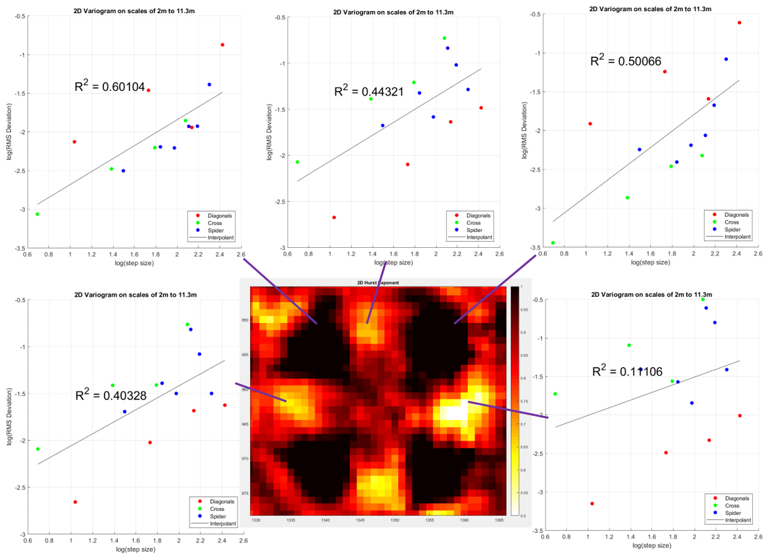
-Similar pattern as above; very high H values (~1) at corners (black) occur due to there being a large difference between the diagonal-arm RMS deviations at small lags (low, since only a segment of a diagonal-arm will show a difference, and a small difference at that) and that at large lags (high, as almost the entirety of the one diagonal-arm will show a difference)

-Very low values of Hurst exponent at orthogonal variogram positions explained by large discrepancy between slope of cross-arm (high slope, corresponding to large change in roughness with scale) and slope of diagonal-arm (low, slope, corresponding to small change in roughness with scale)

 

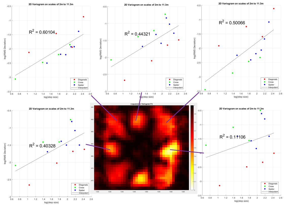
-16-fold symmetry can be explained by directional discretization error: at each of the 8 locations with small r^2 values, there are large deviations in RMS slope (ie. y-intercept on variograms) of diagonal-arm plot lines vs. cross-arm plot lines. Meanwhile, the 8 locations with large r^2 values between them (brown) have relatively uniform RMS slopes amongst diagonal-arm/cross-arm plot lines (and therefore relatively good least-squares fits), since only 1/8 of the spider-arms overlaps with the central depression.

-Meanwhile, the r^2 values in the centre are high owing from their being relatively isotropic, overlapping significantly with the central depression

 

 

 

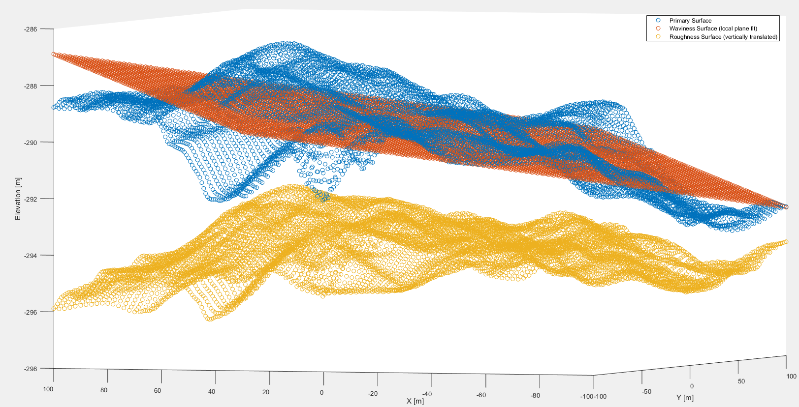
III: COTM LiDAR Roughness Pre-processing 

New COTM LiDaR DEM – 3D Roughness Characterization

 

The plots below show sample variograms, accounting for the

 

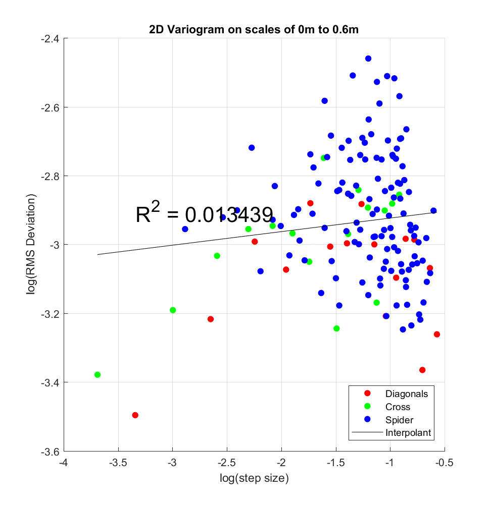
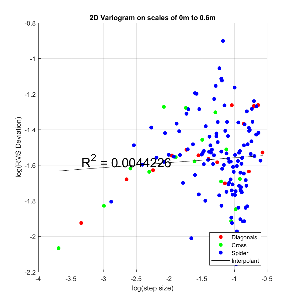
On the basis of the above variograms, there appears to be a breakpoint at approximately -2 on the log x-axis, corresponding to 13.5cm. For step-sizes above this approximate threshold, the linear relationship (in log-log space) between RMS Deviation and step-size -and which is the fundamental assumption for the method employed thus far to calculate the Hurst exponent- no longer appears to hold, with RMS Deviations exhibiting substantial scatter for any given value of step size. An alternative explanation could be that, above the 13.5cm threshold, scale-dependent anisotropy results in the large scatter at given step sizes. To test this, one could colour-code the points by direction (for instance, with respect to azimuth from an arbitrary reference direction), in order to ascertain whether the points in a certain direction tended to show linear relationships. Even were this alternative hypothesis to be validated, however, one would still not be able to explain the anomalous points with low RMS Deviation and large step size.

As such, I chose to limit the range of step sizes to 2.5-14cm (ie. 1-4 pixels, since resolution is 2.5cm/pixel, and the largest diagonal step-size will therefore be 10cm*sqrt(2)=14cm).  The results for 2 choices of cell-size are shown below:

a) Cell size of 81×81 (ie. 2.025 x 2.025 metres)

b) Cell size of 17×17 (ie. 4.25 x 4.25 metres)

It is apparent that whereas in (a) (ie. for larger cell size), though large-scale roughness/smoothness is captured in the RMS Slope map (particularly the almond-shaped central smooth plains), the familiar plus-shaped artifacts present in the roughness maps of Ina D Caldera are likewise present on the COTM map, while for (b), these artifacts are sufficiently small (ie. lower signal-noise ratio, where the artifacts are the ‘noise’ in question) that the RMS slope map delineates the ridge visually evident on the high-pass Gaussian filtered DEM.

Here’s a high-resolution image showing how the RMS slope algorithm appears to track small-scale ridges (ie. on the scale of ~10s of cm)