I: Preliminaries

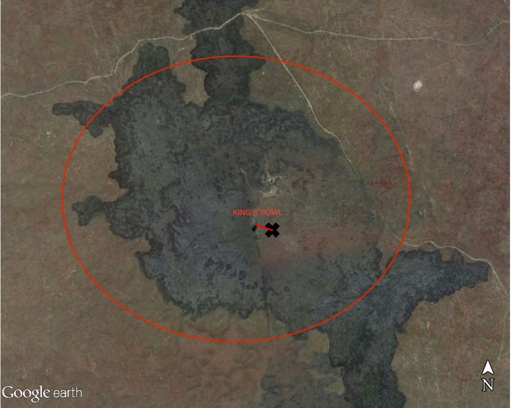
I’ve been doing further work on classifying the spatial distribution of and relationships amongst the mushrooms in Kings Bowl . In particular, I’m testing the hypothesis of whether there’s a bias in their elevations towards lower elevations – where this bias is with respect to the larger population of elevation values throughout the lava pond at Kings Bowl (approximately coincident with the extent of the circle below).

While this may seem qualitatively apparent given the map below, given the apparent clustering of mushrooms in the depressions (purple regions), we wanted to make a more quantitative assessment of this bias.

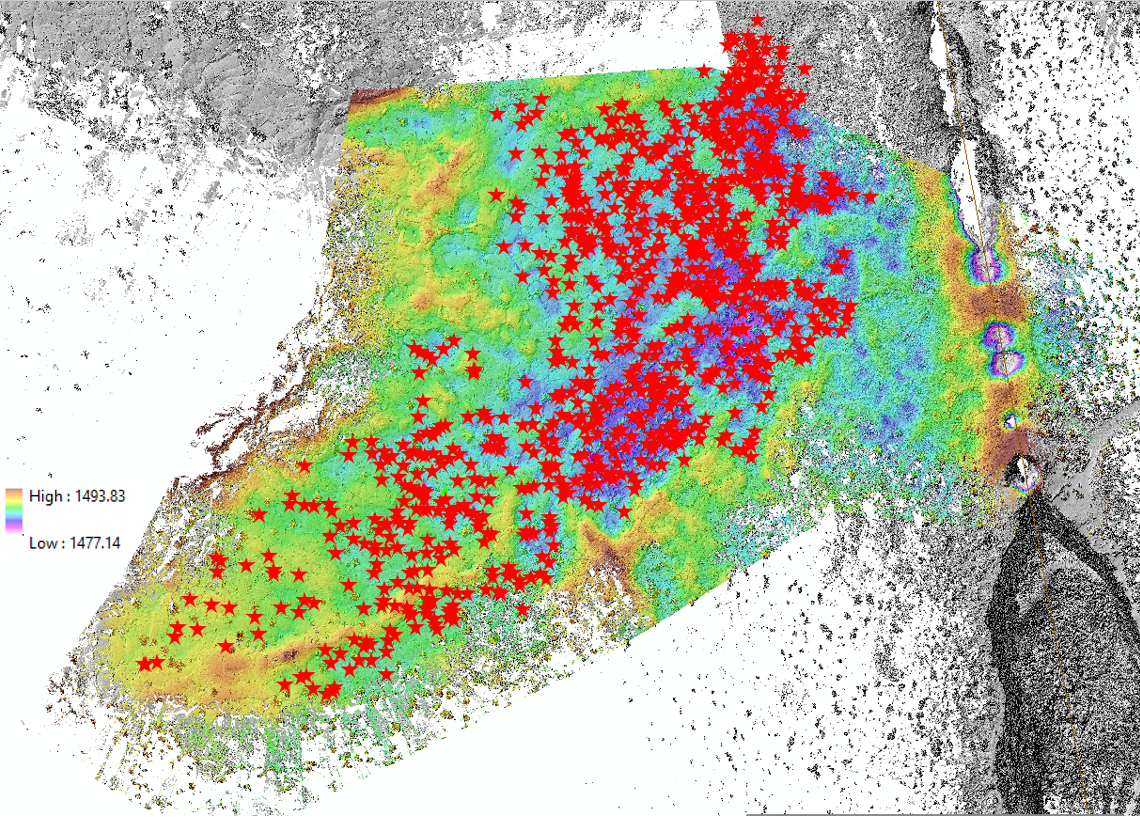
The first step in such a quantitative assessment is thus determining whether we have data throughout the extent of the lava pond. The largest DEM I could find (below), however, had several areas of relatively sparse data coverage (white). For scale, the mushrooms are the small grey/black points in the centre of the map.

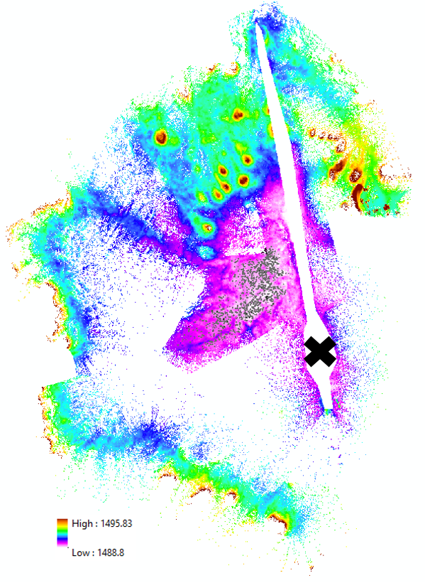
It was also necessary to remove the N-trending linear fissure (the elongate white region extending to the North of the X, where the black X is roughly at the same position as the black X on the Google Earth image above), owing from the fact that it is the origin of, but distinct from, the lava pond. It took me quite some time to figure out how to actually mask out this fissure in ArcGIS – after some frustration, it turned out to be a matter of utilizing graphics -as opposed to vector polygons- by creating a polygon graphic surrounding the entire dataset, then another one encompassing just the linear fissure, and excluding the latter from the former. Even given all of the holes in data coverage, I was amazed that there were still ~200 million points in this DEM.

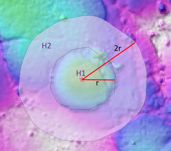
The next step is determining what we actually mean when we say ‘elevation’. For all of the points in the DEM above, this isn’t an issue – however, for the mushrooms, it’s somewhat more arbitrary. I decided to use the ‘background elevation’ H2 of each mushroom (see schematic below) to collate the distribution of mushroom elevations, where H2 is the mean elevation of all the points in the annular region surrounding each mushroom defined by (r,2r). This assumes the mushroom elevation to be the elevation of specifically the bottom of the mushroom. I acknowledge that this is an imperfect measure; for instance, for the mushroom below, the Northwestern portion of the annulus overlaps with what appears to be another mushroom (light blue / green), which will result in a value of H2 somewhere in-between the elevation of this other mushroom, and the elevation of the pink region defining the remainder of the annulus. However, I would consider the pink region alone to be a more representative elevation of the bottom of the mushroom. This bias in the mushroom elevation distribution towards slightly higher elevations (due to this contamination of mushroom annuli with other mushrooms) could have deleterious effects later on for the quantitative assessment we’re trying to perform (to be discussed later on). As the old saying goes, “Garbage in, garbage out.”

One way of reducing the effect of this bias could be to reduce the size of the annuli (such as to (r,1.1r)). However, there would still be some inter-mushroom contamination. To completely prevent the possibility of any contamination, I think that a better method would be to perform a low-pass Gaussian filter of the surface encompassing the mushrooms (the same procedure coincidentally that I’m applying in the 2-dimensional roughness algorithm being developed). The cutoff wavelength to be employed with this Gaussian filter should then be something like 10m*, to ensure that the largest mushrooms (about ~2m in diameter) would be filtered out, leaving a more representative, large-scale measure of mushroom bottom elevation.

*This jibes with the ‘5x’ rule proposed in some surface metrology filtering sources. Since the Gaussian filter has a graduated, rather than a sharp cut-off, if the cut-off wavelength were 2m, ~1-2m diameter mushrooms would still be partially present in the filtered elevation map.

Cognizant of the problems both with the variably-sparse data coverage of the lava pond elevation population, and with the upwardly-biased mushroom elevation population, we nonetheless have two elevation populations to work with, with which we can move on to the quantitative assessment of their degree of similarity.

 

II: Quantitative (Probabilistic) Assessment of Elevation Distribution Similarity: Applying The Anderson-Darling Test 

Dr. Neish proposed that I apply the same method as was used in her paper “Elevation distribution of Titan’s craters suggests extensive wetlands” (Neish and Lorenz 2014): the Anderson-Darling Test, which provides a quantitative measure of the probability with which a sample distribution (mushroom elevations in our case) was drawn from a hypothesized distribution (the elevations of the points comprising the lava pond -minus those comprising the fissure- in our case). In formal terms then, our null hypothesis is that the 2 distributions are probabilistically indistinguishable, while our alternative hypothesis is that the 2 distributions are probabilistically distinguishable.

For the purpose of the Anderson-Darling test, I didn’t clip any edges, mostly because I’m not so sure with this new dataset how much to clip out. In any case, hopefully Dr. Zanetti and I will be able to get more complete LidAR coverage during the upcoming field work, so as to more accurately represent the topography distribution of the lava lake.

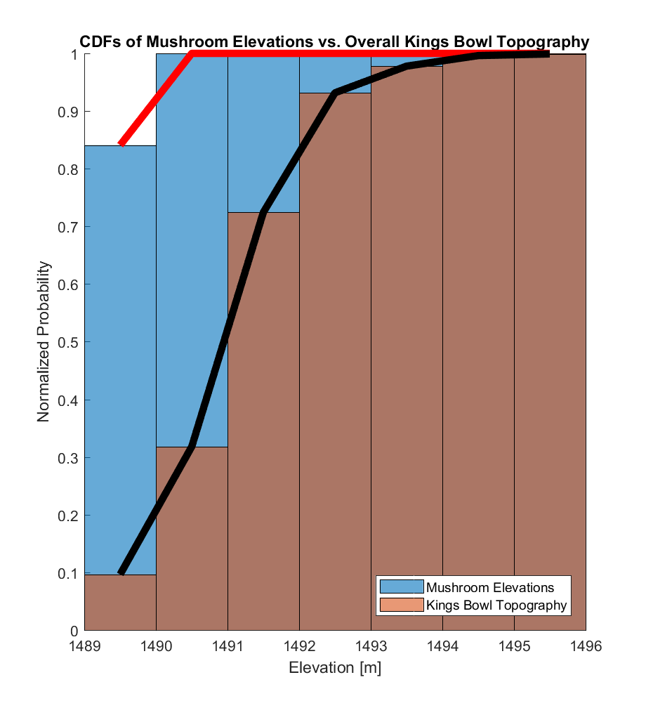
The histograms (formally, the probability density functions (PDFs), such that the areas under these curves are normalized to exactly 1) of these two elevation distributions are visualized below, where the mushroom elevation distribution was calculated from a population of 886 samples, while the kings bowl elevation distribution was calculated from a population of  225,314,122 samples.

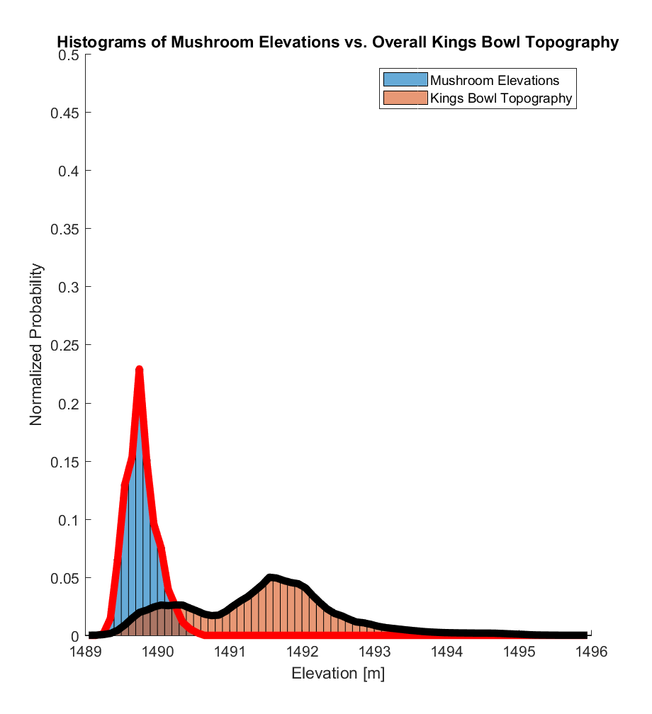
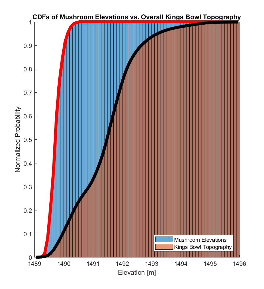
The corresponding CDFs (normalized to maximum values of 1) are visualized below. In both cases, there appears to be a substantial difference between the 2 distributions, with almost all (>99%) of the mushroom elevations being within the range of the lowest ~20% of the overall Kings Bowl lava pond elevations.

The Anderson-Darling test statistic A2 uses these CDFs as inputs, such that

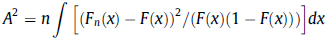
, where n is the number of samples in the specified distribution (ie. ~200 million in this case, for the LiDAR DEM pictured above),

Fn is the cumulative probability function (CDF) of the sample (mushroom) elevations,

F is the CDF of the LiDAR DEM elevations, and

dx is an infinitesimal change in x (the elevation in metres).

 

One way to think about this equation is that the integrand is simply a distance function, measuring the squared difference (or squared residual) between our data (mushroom elevations) and a the hypothesized probability distribution with which we wish to compare this data. The only catch is that the particular ‘weighting function’ used in the Anderson-Darling Test is 1/[F(x)*(1-F(x))], which has the effect of weighting the tails of the probability distributions relatively heavily. This integrand is then integrated (ie. the continuous analogue of summation) over all x-values of the distributions – a procedure typically performed when calculating probability density functiosn, for instance- providing a measure of the how much the 2 distributions differ, at each and every one of their x-values. The result is finally multiplied by n, resulting in A2.

 

In discrete terms amenable to numerical computation, I interpret this equation as

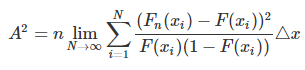
where F, Fn, and n are as before, while

x is the set (union?) of all x-values at which the CDFs of the 2 distributions are sampled*

i is the summation counting variable,

xi is the ith elevation bin of the CDF (of F or Fn),

N is the maximum value of the summation counting variable, and

Δx is the elevation bin width (presuming equally-spaced bins).

*In this case, both elevation distributions are restricted to the domain [1489,1496] m.

 

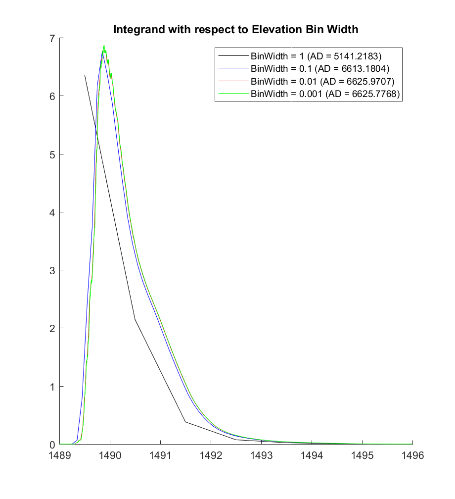
Since we can’t in practice use infinitely many infinitesimally small elevation bins, I exponentially increased the number of bins (or equivalently, exponentially decreased the bin width) in powers of 10, in order to see whether the integral would converge to some value. For instance, for a bin width of 1m, there are only 7 bins; while for the CDF plot above, the bin width is 0.1m, resulting in 70 bins for each distribution.

The plot below displays the value of the integrand (of the above discrete A2 equation) as the bin width is iteratively decreased, and it visually suggests convergence at smaller and smaller bin widths.

 

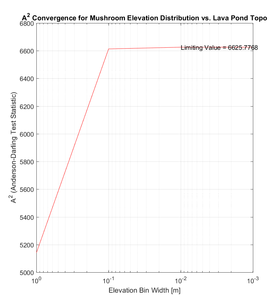
The corresponding values of the Anderson-Darling (AD) test statistic A2, for each bin width, are shown below. In this particular method, the integral (ie. the area under the above curves) is calculated via the trapezoidal numerical integration method, in which the area under the integrand is partitioned into trapezoids at equally spaced x-intervals.

 

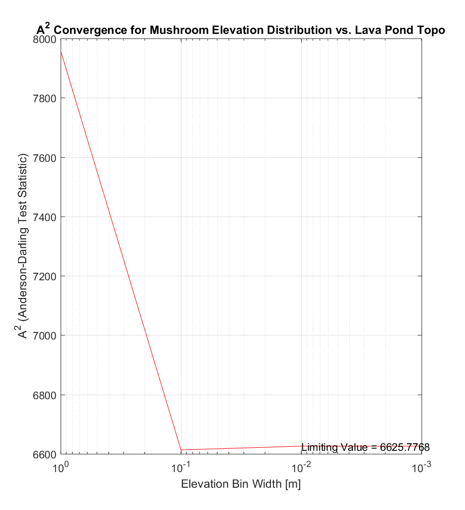
In an attempt to corroborate the use of the trapezoidal method, I also performed numerical integration using the more conventional method of Riemann summation with rectangles, with the midpoint rule (ie. using rectangles with height equal to the value of the integrand at points half-way between bin edges) as shown below.

 

The resulting values of A2, while dissimilar for large bin widths, nonetheless converges to virtually the same value of A2  as for the first method (~6625.8), suggesting a robust estimate of A2.

However, I am not sure about how to proceed to calculating the p-value (ie. probability of the null hypothesis being correct, ie. that the mushroom elevations are drawn from the lava pond elevation distribution), as this was not clear in the paper “Distribution of the Anderson Darling Statistic” (Lewis 1961). In particular, the meaning of the independent variable ‘z‘ in F(z;n) was not explained. Determining the p-value looks like the last step in ascertaining the likelihood of the aforementioned null hypothesis, and by corollary whether the mushrooms in Kings Bowl are preferentially distributed at the lowest points within the lava pond.