I’ve spent much of the past little while editing an (extended) abstract, for planned submission to the coming LPSC conference in January. This has been surprisingly difficult – perhaps owing from the fact that I had originally written a 6-page abstract, which needs to be pared down to 2 pages as per the formatting requirements of the conference. Fortunately, I think I’m nearly there – though it’s required a lot of thinking on what is really important, and what is more of a footnote. Most of the methodology concerning the roughness method fits along the lines of the latter, as I’m guessing most potential readers aren’t so interested about, say, the exact formula used to derive the maps for RMS Slope and Hurst Exponent, nor the details of the 3-dimensional Gaussian Filter, which I’ve thought so much about and spent quite a bit of time implementing myself in MATLAB, to ensure that I really understood what going on in the filtration process.

 

I) More Rubbly Flow Plots 

I’ve also spent the past little while taking a closer look at the Rubbly Flow LidAR DEM from the 2016 field season at COTM. In particular, assuming we evaluate the RMS Deviations derived from the lags between all points within the entire,  I’m interested in seeing whether the size of the Gaussian filter employed (ie. the cut-off wavelength at which 50% of the spatial topographic signal is transmitted and 50% is attenuated) had any appreciable effect upon the final roughness parameters (RSM Slope and Hurst Exponent). I’m also interested in seeing the extent over which the scale-dependent ‘correlated roughness’ behaviour noted previously (in my last blog post) holds: the scale threshold below which we have anisotropic roughness, and above which there is no longer any appreciable correlation between the heights of point pairs within a DEM.

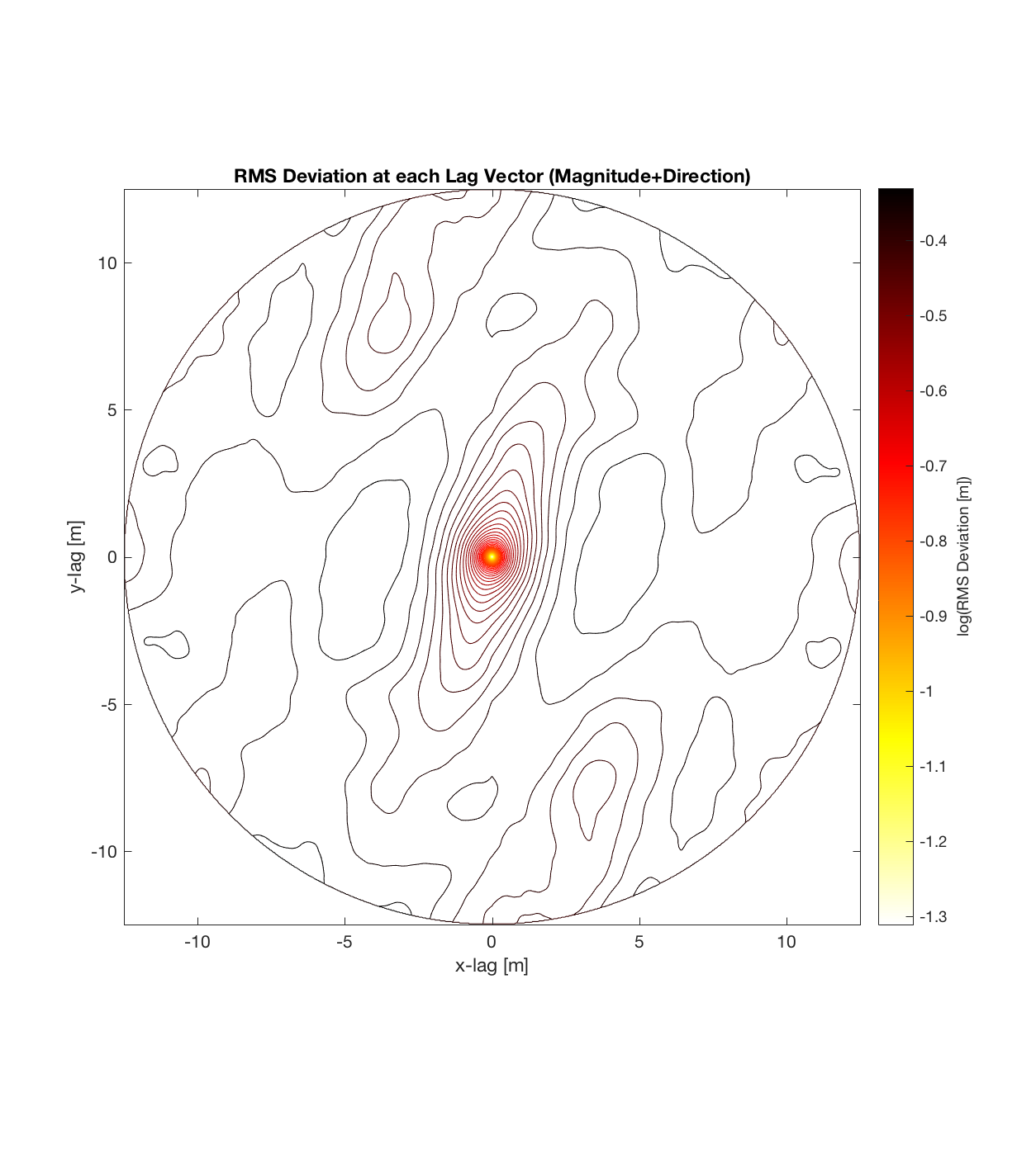
The plots below show the Gaussian filtration process for a cut-off wavelength of 6.25m, followed by the contour plot of the RMS Deviations given all combinations of lag vector magnitude/direction, in both the x and y directions, from scales of 0.025-20m. This is essentially a 3D ‘variogram surface’, as opposed to a 2D ‘variogram curve’, which would just be a profile along a particular direction within this surface. As previously observed, the contour plot shows an apparent preferential ‘smoothness’ direction about 20 degrees clockwise of North. This is also the direction in which the RMS Deviation contours change most slowly, implying that this is the axis of minimal Hurst Exponent (small rates of change of RMS Deviation with respect to scale indicate a small Hurst Exponent; large rates of change of RMS Deviation with respect to scale indicate a large Hurst Exponent). Conversely, the direction perpendicular to this, at about 110 degrees clockwise to North, is the axis along which the RMS Deviation contours change most rapidly, and is consequently the axis of maximal Hurst exponent. I infer that the former, aligned along the (principal) axis of minimal Hurst Exponent, at 20N, is the flow direction in which the rubbly flow was originally emplaced.

Furthermore, the threshold scale segregating isotropic/anisotropic behaviour (ie. circle vs. ellipse) is ~1m, as previously observed to be common for COTM DEM’s, while the correlation threshold ranges from 2-10m (in magnitude), varying with respect to direction. I think this indicates that use of the 3D RMS Deviation contour plot is important in variogram analysis; because if we subsequently choose to make variogram profiles (cuts) along particular axes of this surface, the contour plot tells us (at least qualitatively – haven’t yet worked out quantitatively) where to expect a breakpoint to appear – which is to say the range over which a 2D, conventional variogram analysis that assumes a linear log-log power law relationship should hold.

Another interesting thing this large-scale plot shows (I believe the largest I’ve used yet – difficult to do in general due to computational limitations!) is that once we’ve reached the correlation threshold, RMS Deviation doesn’t significantly increase after this – as is indeed predicted by most variogram models, in which RMS Deviation (just the square root of semi-variance, the statistical measure more commonly employed in geostatistics) increase asymptotically. (The exponential and Gaussian variogram models exhibit this asymptotic behaviour, while in the spherical variogram model, the RMS Deviations actually attain a maximum value for a sufficiently large lag, denoted the ‘range’. [Bohling 2005: “Introduction to Geostatistics and Variogram Analysis”]). This asymptotic value appears to be approximately log(-0.5) for this contour plot, which is an RMS Deviation value of about ~0.3.  For lags outside the anisotropic ellipse

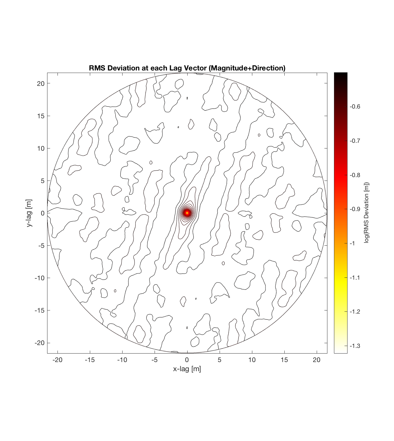
(I unfortunately forgot to save the variogram associated with this contour plot)

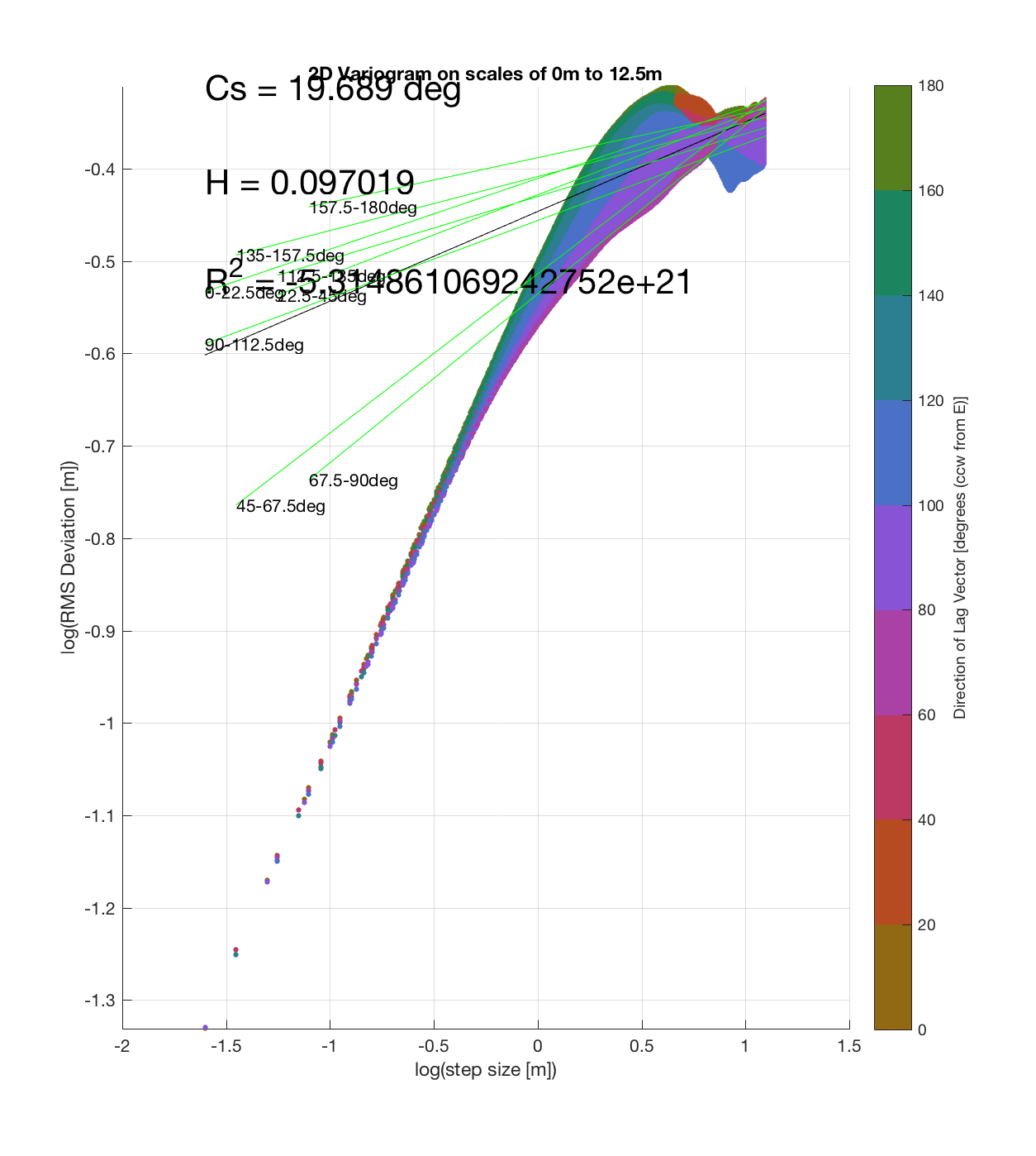
I also tried using a smaller area but a larger Gaussian filter (cut-off wavelength of 12.5m, instead of 6.25m), which resulted in the following RMS Deviation contour plot and variogram. Upon comparison with the variogram for the smaller Gaussian filter used above, the flow direction appears to be the same, in addition to the approximate correlation threshold (2m in the x-direction). I should perhaps do some coding however to automatically calculate the 2 principal axes, so that I’m not just making these 1st order estimates of flow direction, isotropy/anisotropy threshold, and correlation threshold. Meanwhile, the variogram corroborates the contour plot, as there is isotropic behaviour from the minimum scale (0.025m) to ~1m -manifested by the fact that all RMS Deviations for all lag vectors graph as approximately the same linear relationship over this scale- and anisotropic behaviour from ~1m to 6m (the maximum scale used) -manifested by the divergence of the lines with respect to direction over this scale range. Finally, above this scale (lag of 6m = log(0.8) on the variogram), we see the ultimate transition: the correlation threshold, above which all point pairs heights are essentially uncorrelated, such that there is neither an isotropic nor anisotropic relationship, RMS Deviations attain a maximum / asymptotically maximum value despite increasing lags beyond this threshold, and the surface is maximally ‘rough’.

 

 

 

 

 

II) Exploring Aristarchus 

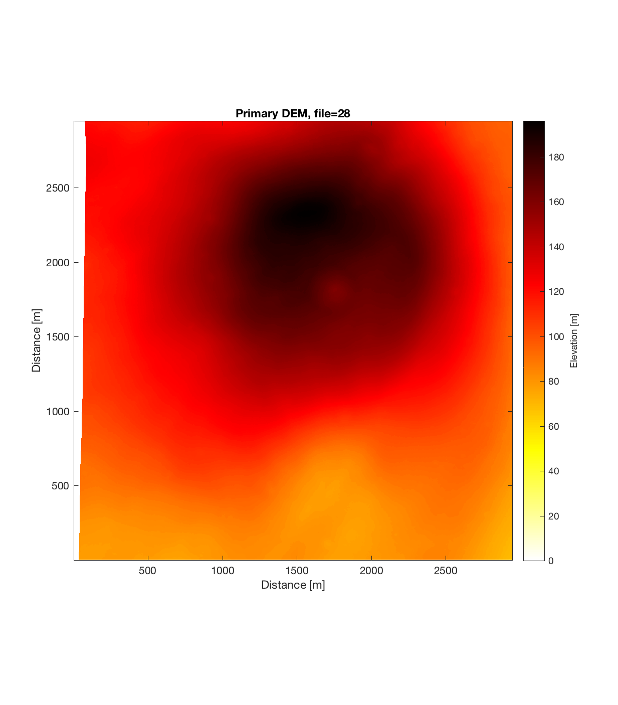
I also explored an LROC (Lunar Reconaissance Orbiter Camera) DEM, which Catherine recommended doing. I randomly chose a DEM of Aristarchus (http://wms.lroc.asu.edu/lroc/view_rdr/NAC_DTM_ARISTARCHU5), with 2m/pixel resolution:

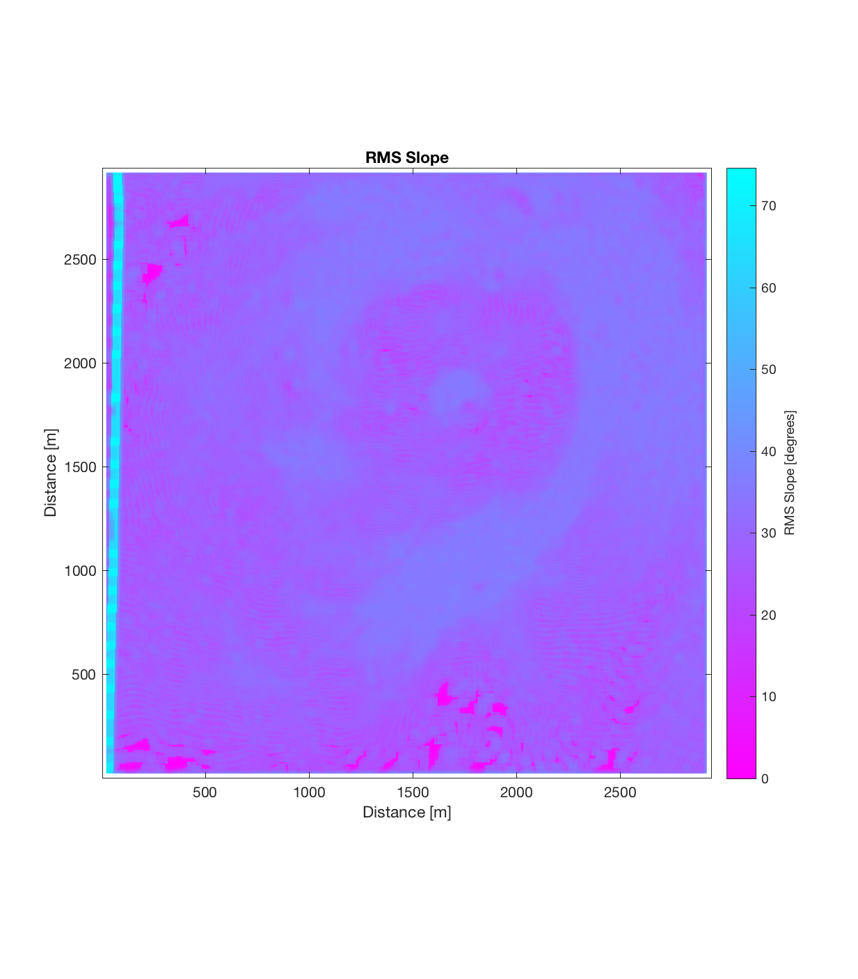
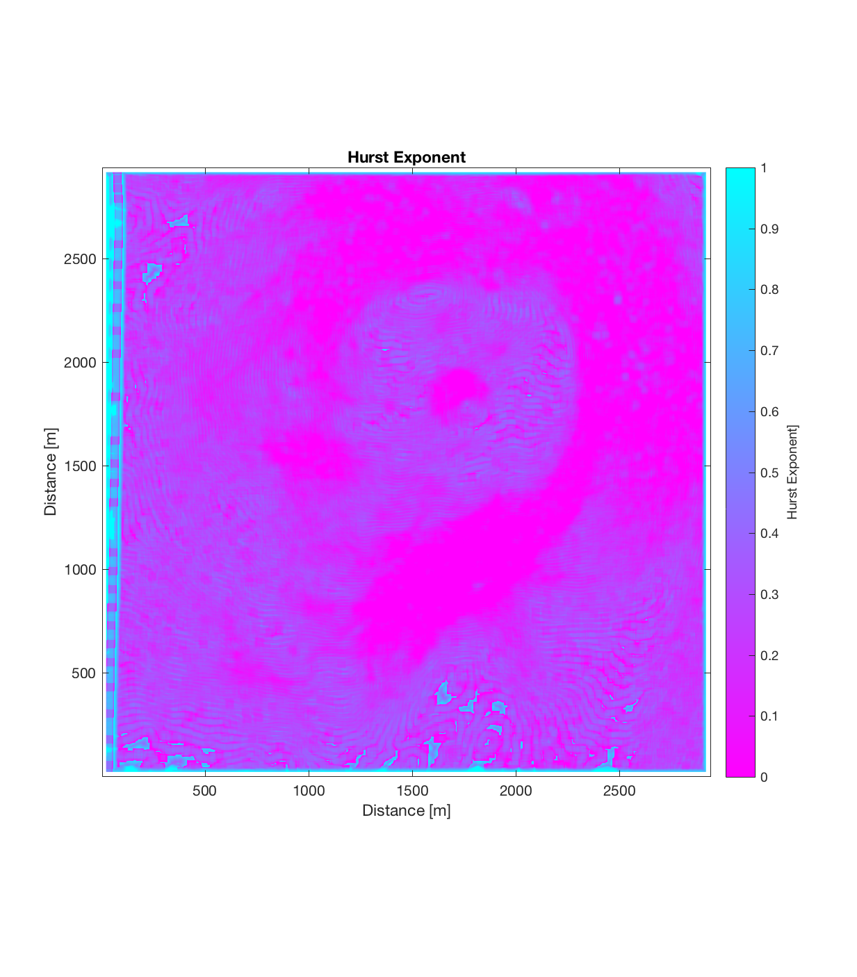
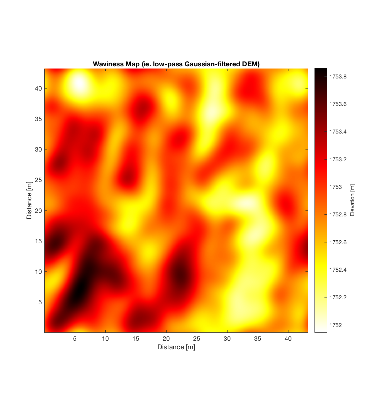
Running this DEM through the roughness code, with a Gaussian filter cut-off wavelength of 50 m, scale range of 2-12m, and cell-size of 42x42m (ie. 21×21 pixels per cell), produces the following plots:

 

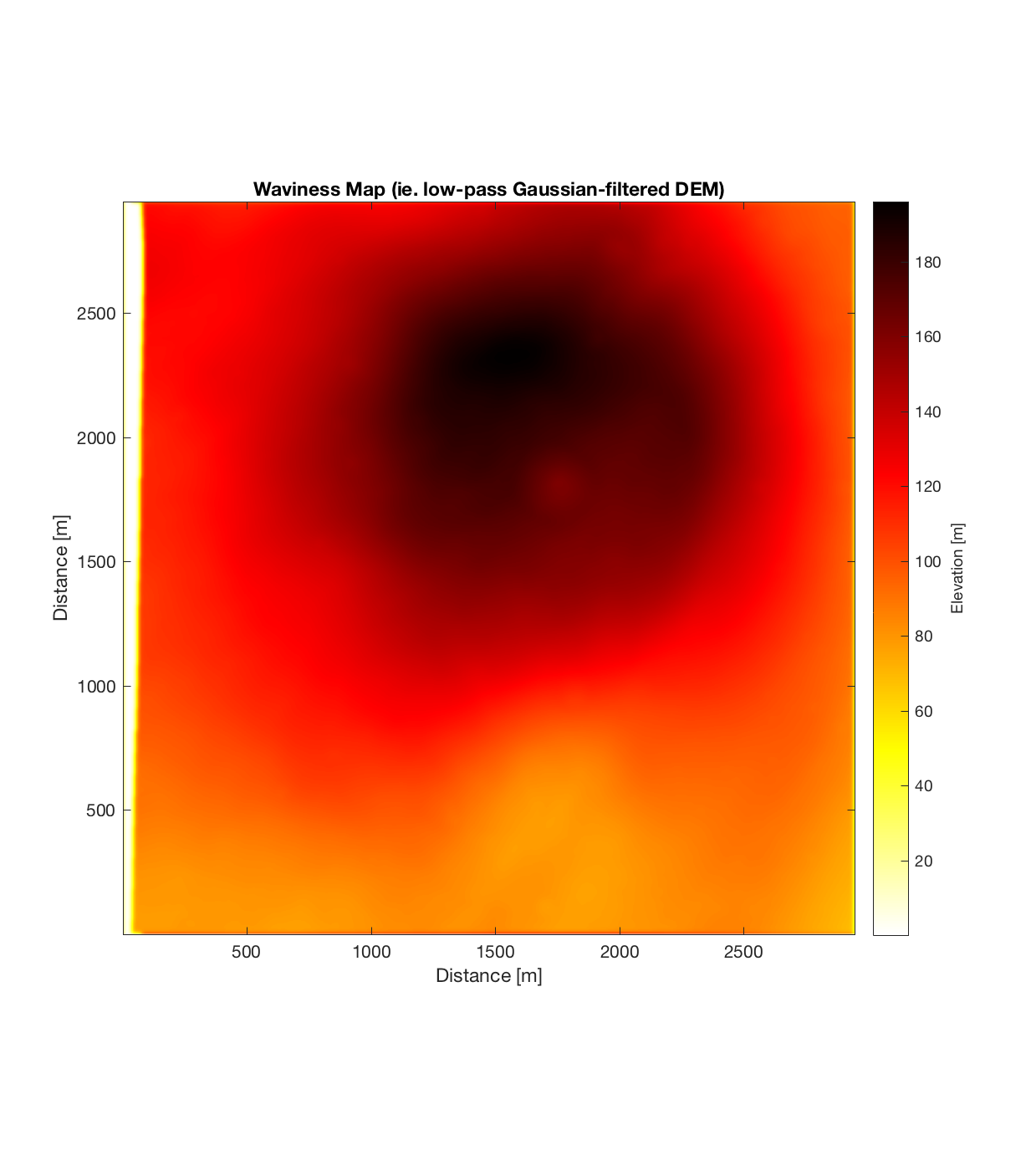
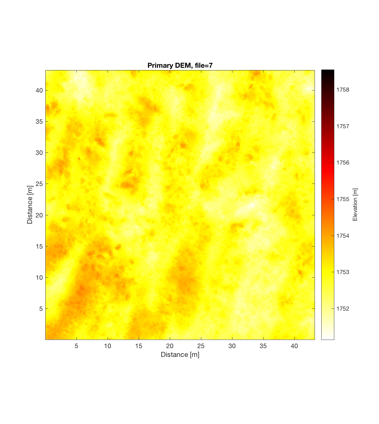
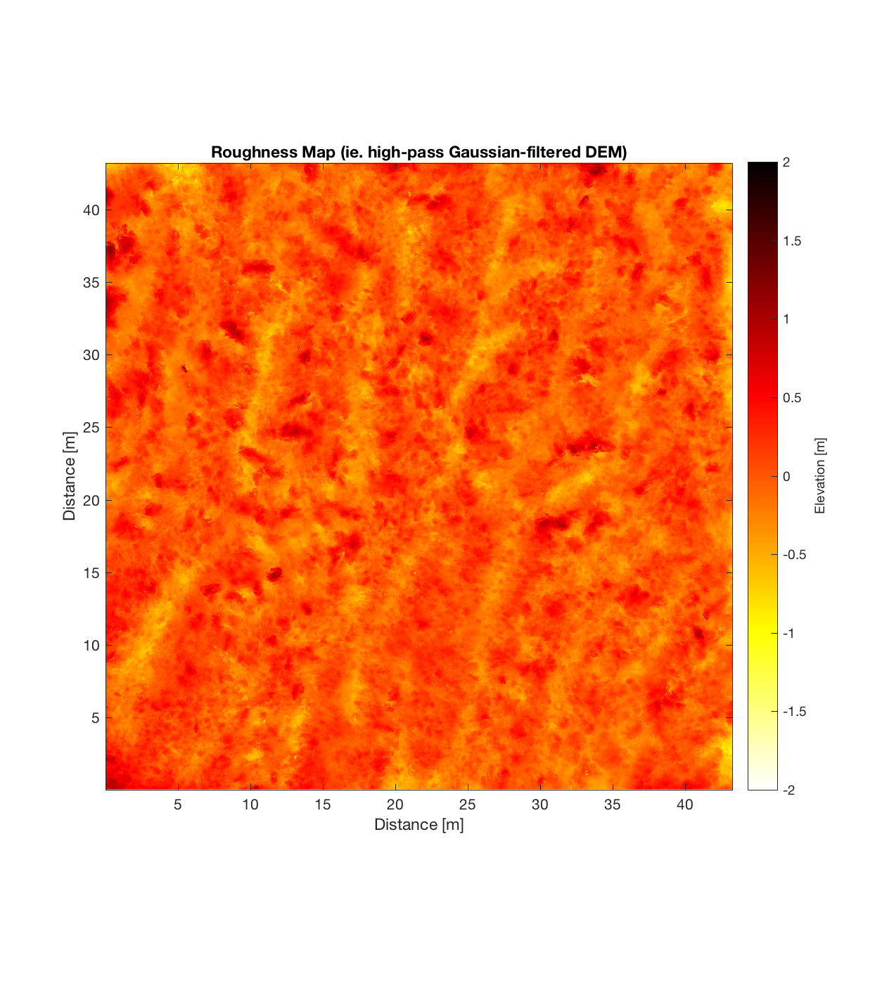
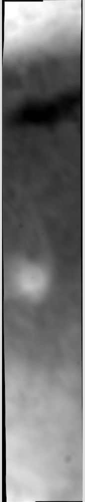
Having subtracted the large-scale topography (waviness), the resultant roughness DEM is quite interesting, possessing an intricate, sinuous small-scale structure:

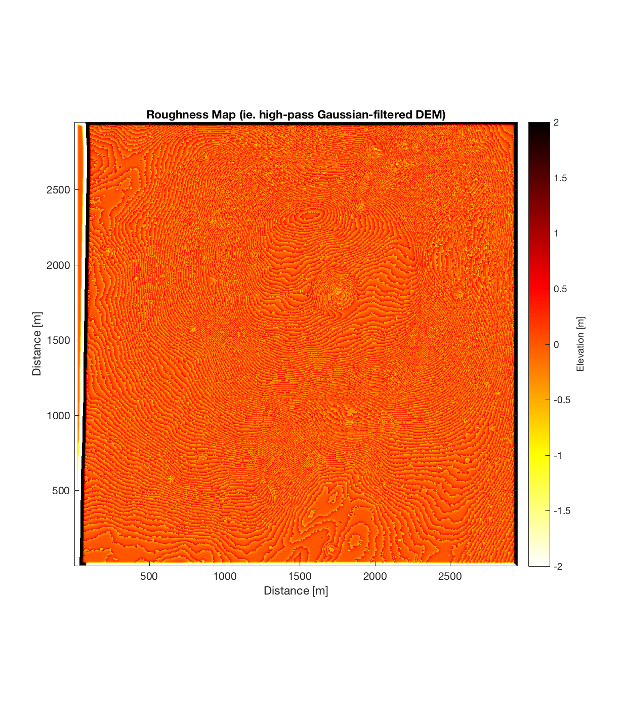
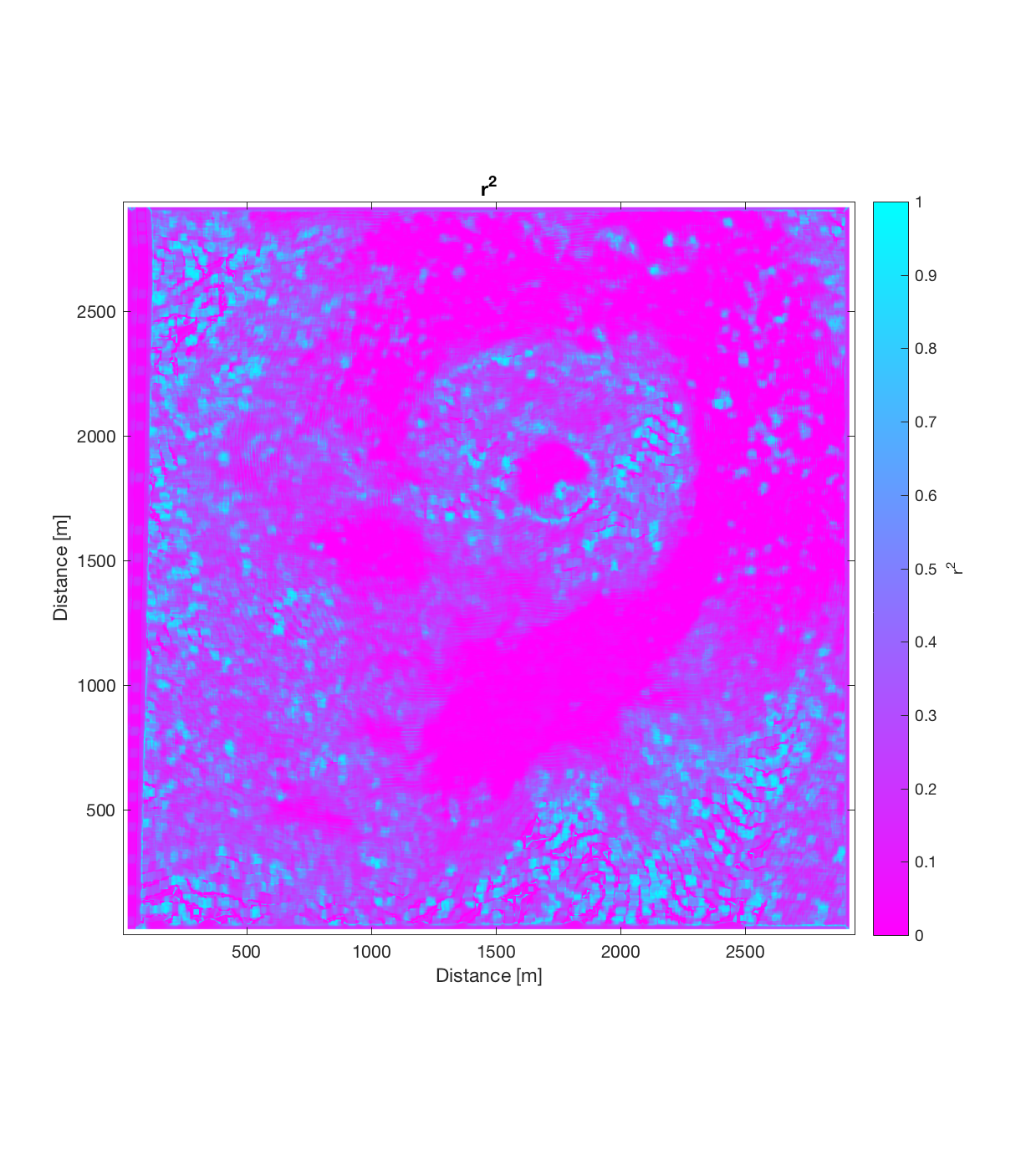
The RMS Slope and Hurst Exponent plots also show some large-scale structure, with a roughly circular region of lower RMS Slope (~25 degrees) and higher Hurst Exponent (~0.4) centred around (1750m, 1750m) in the DEM, surrounded by a region of higher RMS Slope (~40 degrees) and lower Hurst Exponent (approaching 0). I find this interesting, because even though it ostensibly appears the circular, positive topographic anomaly has been removed by the application of the Gaussian filter (ie. such a circular anomaly can not be discerned in the roughness DEM above), both of these roughness maps show the signature of this region. Perhaps this implies therefore that this circular region was produced by different geomorphic process than its surroundings. Of course, the strength of such an assertion is weakened by the fact that the r^2 plot (the final plot below) generally shows extremely low r^2 values, approaching 0 for the region surrounding the circular anomaly. This very low r^2 value could be due to rapid, fine-scale changes in roughness direction within this surrounding region: which is to say a high degree of anisotropic roughness.