Nearest Neighbour Index

By using the nearest neighbor index tool in ‘CrimeStat’, residential break-ins (B&E’s) were found to be less spatially aggregated than auto thefts, however commercial B & E’s are similarly spatially aggregated to auto thefts. The index tends to increase quickly as the nearest neighbour order increases, then starts to level out as it reaches the last nearest neighbour order. The graph in Figure 1 depicts that residential B & E’s are less spatially aggregated, and therefore more random because residential areas are not particularly ruled by laws as strongly as commercial areas. Commercial areas display higher spatially aggregated B & E’s, which may be due to land use and zoning regulations which force these areas to be closer together. This leads to a higher spatial aggregation in B & E’s for commercial properties. Auto thefts are more spatially aggregated than residential B & E’s and shares a close nearest neighbour index to commercial B & E’s, which may be related to parking lots or areas where there are large amounts of un-attended cars. These parking lots are areas more commonly targeted by thieves, and typically exist in commercial areas which are not as randomly distributed.

Moran’s Index for Spatial Autocorrelation

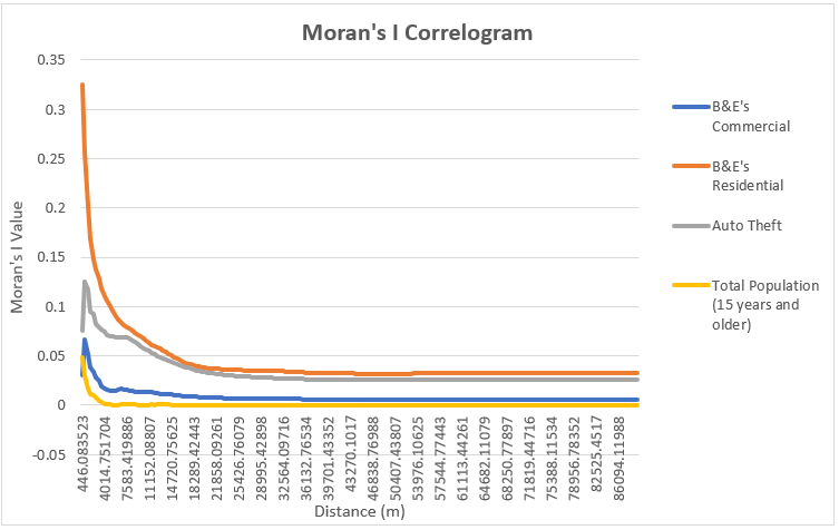
The Moran’s Correlograms tell us how spatially clustered the Moran’s I values are, and how spatial auto-correlation changes when moving away from a point. (Levine, 2010). The nearest neighbour index compares the differences between nearest points and distances that would be expected based on chance and to see if values are clustered, dispersed, or random. Moran’s I Correlograms on the other hand provides information about the scale of spatial auto-correlation, and whether these values are concentrated near each other or diffuse moving away from a point. Commercial B & E’s and Auto theft both show similar curve shapes in the Correlogram, where the crimes are most spatially autocorrelated around 800m to 1300m away from existing crimes. It could be speculated that this is because thieves do not want to work in immediate vicinity of previous or other crimes as it might be too easy for them to get caught, however they may still want to work in the same area that they are familiar with. Residential B & E’s however have the highest spatial autocorrelation within the immediate vicinity, which may show that thieves prefer to target multiple houses within the same street or neighbourhood. Not all crimes are distributed the same as the population values, indicating that population doesn’t explain crime distribution.

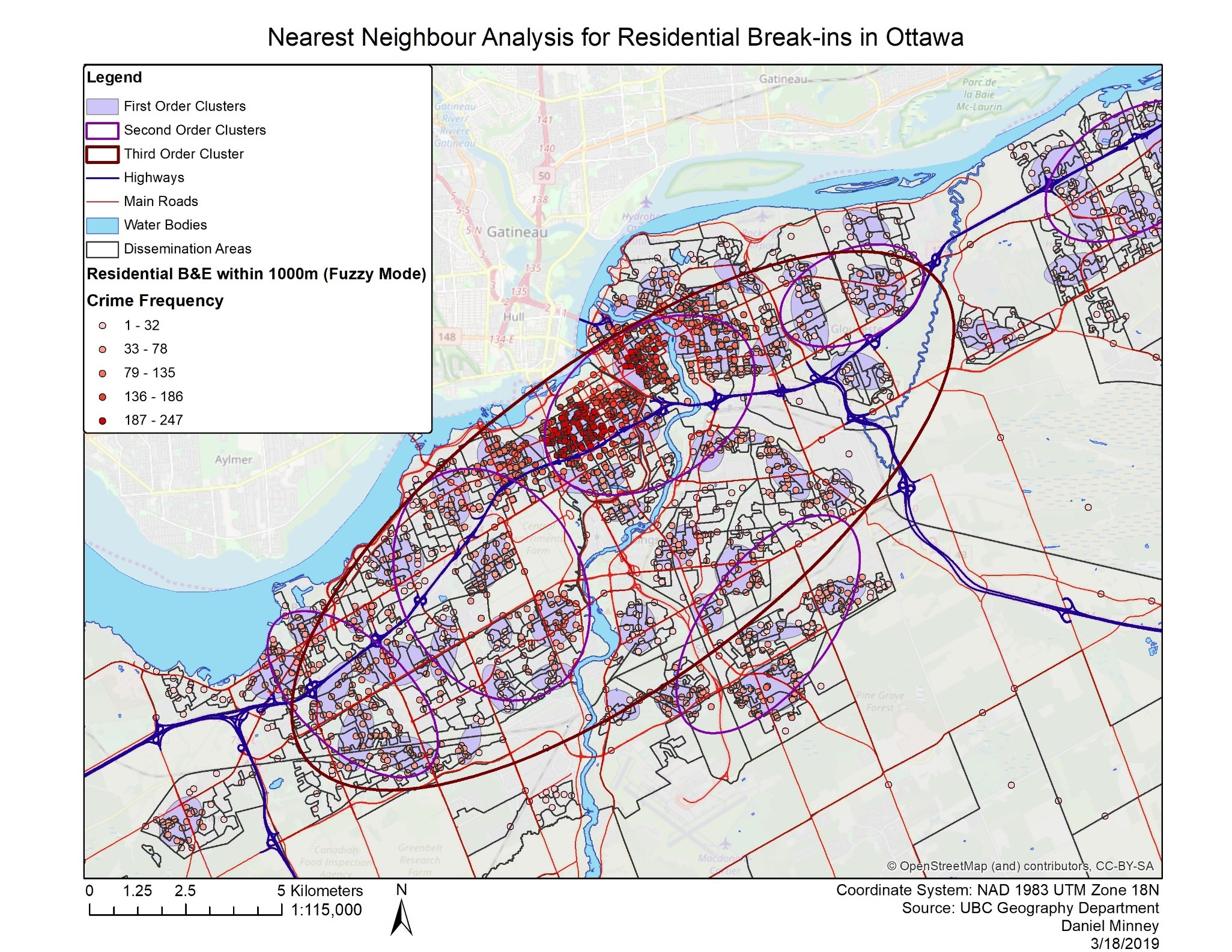
Fuzzy Mode Clusters and Nearest Neighbour Analysis

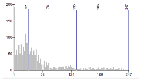
Using fuzzy mode clusters for residential B & E’s, normalized by population, a map was produced that displays the frequency of crimes within a 1000m radius of each point. The lowest frequency class is between 1 – 32 crimes, and the highest is 187 – 247, as seen in Figure 4: Nearest Neighbour (fuzzy mode) Analysis. The histogram shows that the data is right skewed, however since higher values represent more frequency of crimes near a point on the map, this is not particularly useful.

The mean of the data is 52, however the standard deviation is 53, which means that the data is highly variable. By looking at the map, it can be depicted that a large amount of high frequency crimes occur in the central area of Ottawa, which may be expected in most cities. More importantly, it seems that a large amount of residential B & E’s occurs along or near to a highway. This may indicate that criminals prefer to target houses located along a highway as it makes for an easy and efficient escape route. Missing information for Quebec may also provide additional context as a lot of the high frequency points are located near the provincial border with Quebec just on the North side of the Ottawa river.

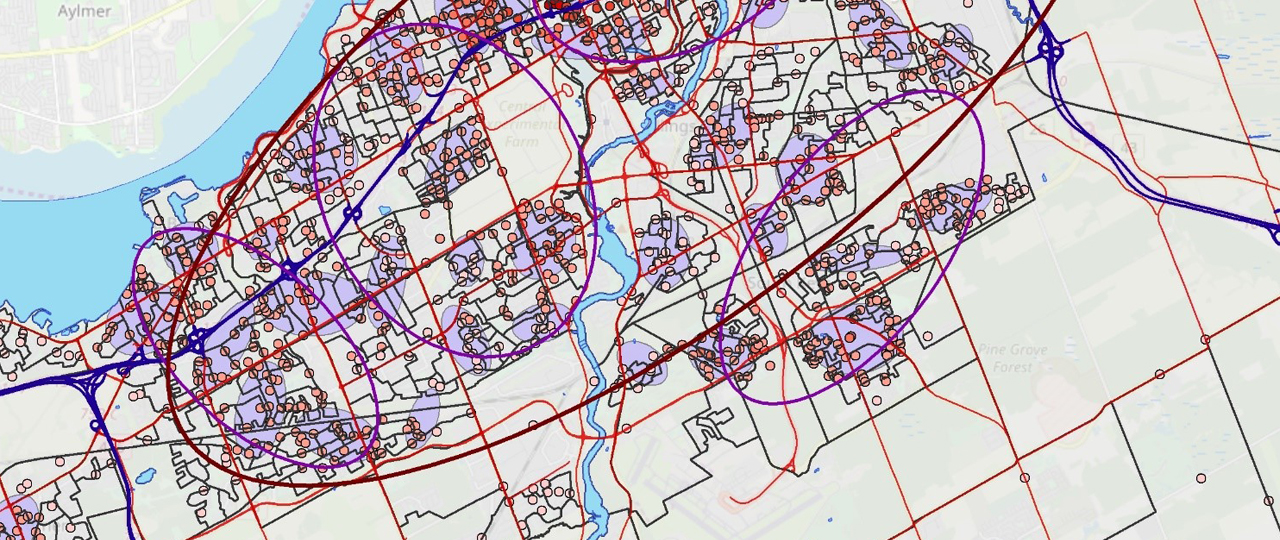
                The clusters provided using the nearest neighbour hierarchical spatial clustering paint a different picture. As opposed to the fuzzy mode clusters, these seem to be more evenly distributed across the city, seen as purple ellipses in Figure 4, and do not show any spatial trends regarding the downtown core of Ottawa or city features such as highways. These purple ellipses are created through two or more points that are closer than the nearest neighbour distance (Leitner, 2013). The nearest neighbour hierarchical spatial clustering does mostly contain the points created from the fuzzy mode analysis, yet the shapes of the ellipses seem to be random.  Risk adjust nearest neighbour analysis was then conducted to produce second and third order clusters, where cluster centres are treated as points, and are themselves clustered. (Levine, 2010). Risk adjusted analysis considers the density of population above the age of 15, which is associated with those more likely to commit crimes. However, this presents a more general idea of where residential B&E’s occur in the city. The third order cluster produces only one cluster as it is the final cluster that can be computed, showing that crimes mostly occur in the central area of Ottawa, which is likely due to the higher population density in this area.  

Auto Thefts and Space-Time Relations

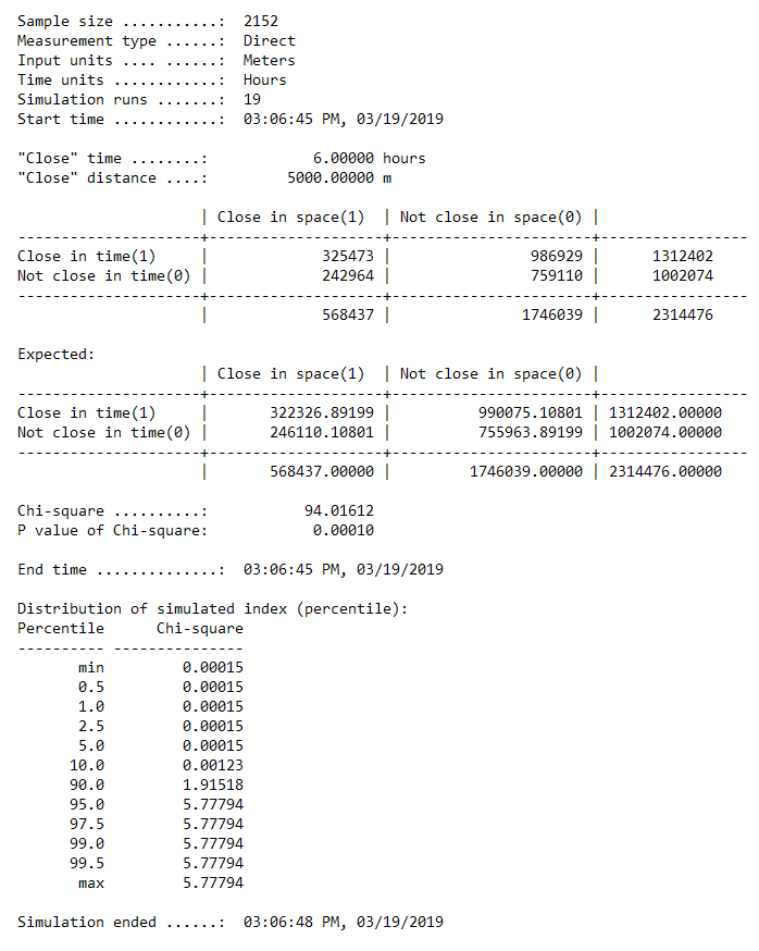
Although spatial clusters provide useful information into spatial trends for crimes, temporally, it is expected that certain crimes occur during certain times of the day. Levine describes this as a clustering of crimes in time (2010).  The Knox index approach was used, which assess both clustering in space and time, and compares their relationship with each other (Knox, 1964). Auto thefts were analyzed using the Knox index to see if their occurrence in Ottawa is related to time and space in which they occur. Overall, there are a large amount of auto thefts that are close in space and time, more than is expected than if auto theft was distributed randomly throughout the city. This may suggest that auto thefts are committed in a similar time frame, particularly when people are at work or asleep at home and have left their cars unattended outside in areas where there are no parking garages for houses and apartments. Additionally, a large amount of auto thefts was similar in space but not time, suggesting that these types of crimes may occur in the same areas of the city, but not always at the same time of the day. These areas could consist of concentrated parking lots that are not patrolled, such as those mentioned previously.

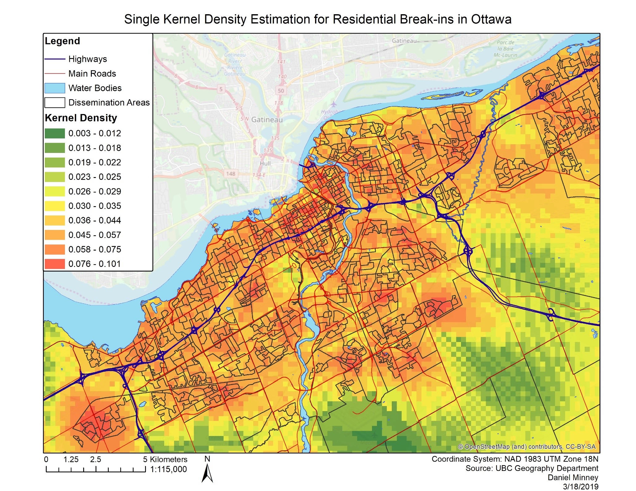
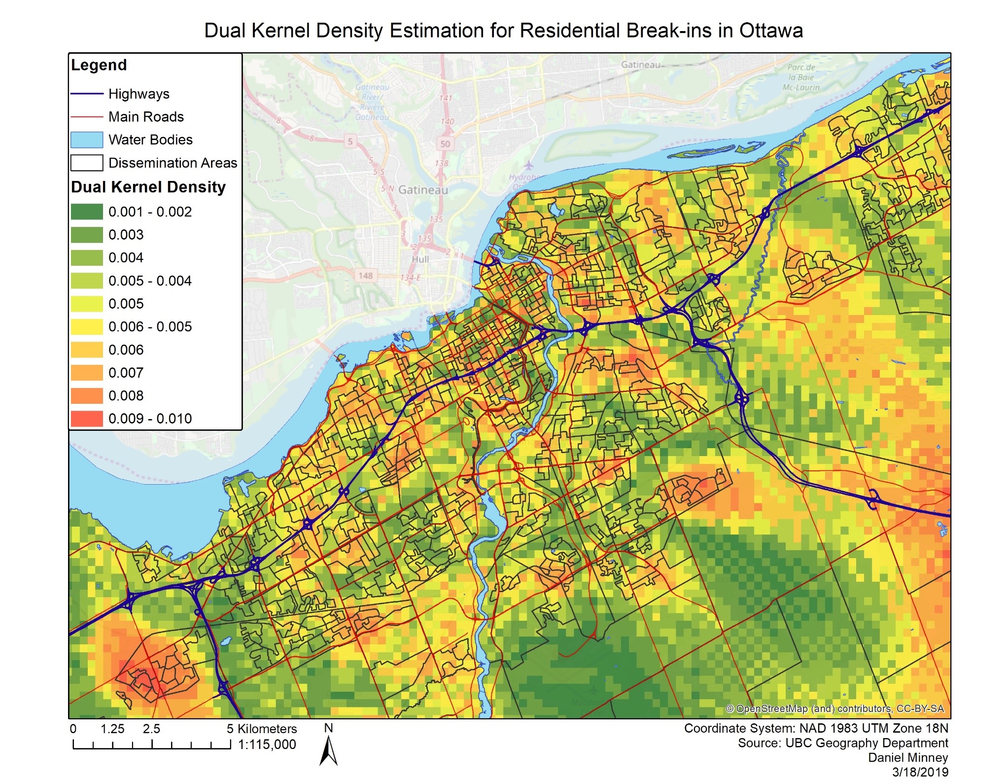
Interpolating Residential B&E’s in Central Ottawa

The smooth point estimates created using the Kernel Density tool provides a surface that displays a continuous surface of crime density across the city of Ottawa as opposed to hot-spot analysis which provides clusters of frequent crimes (Levine, 2010). Kernel density estimates are preferred over other types of interpolation such as kriging because it is more appropriate for single point locations (Levine, 2010). The results provided by the Kernel density estimate (KDE) offer a broad understanding of where high amounts of residential break-ins occur across Ottawa, but no real definition is provided as most of central Ottawa displays a density of 0.036 or higher (seen in Figure 6). Additionally, areas that contain By normalizing the KDE using population over the age of 15 years, more context is provided. This allows for the visualization of areas that experience high amounts of residential break-ins compared to the population density in the area. As seen in Figure 7, the highest density area is outside of the central area of Ottawa in Kanata, contrary to previous findings. Yet, there are still some high-density areas within central Ottawa, but a large amount of the high density found in the single KDE has been reduced with the normalization. It is important to understand that population over the age of 15 may not be an appropriate variable for normalizing residential break-ins, but it does provide some context on how different variables may affect the results of a kernel density estimate and may be useful in further crime mapping techniques.  Additionally, Levine notes that kernel density estimates are limited by their overgeneralization of data, mainly due to a resolution problem, where the resolution of the data being estimated likely lower than the resolution of the cells produced (2010). Additionally, a concentration of crime in one area, such as auto thefts being concentrated in parking lots, may be generalized and bleed over into areas such as residential ones that do not experience high amounts of auto theft. The plethora of options and settings when setting up the CrimeStat tool also make it unlikely that the most accurate settings are always selected.  Although these problems may be present within the results, the kernel density interpolation method generally works well at the city scale.

Maps

Works Cited

Knox, E. G., & Bartlett, M. S. (1964). The detection of space-time interactions. Journal of the Royal Statistical Society. Series C (Applied Statistics), 13(1), 25-30. doi:10.2307/2985220

Leitner, M., & SpringerLink ebooks – Earth and Environmental Science. (2013;2012;). Crime modeling and mapping using geospatial technologies (1. Aufl. ed.). New York;Dordrecht;: Springer.

Ned Levine (2010). CrimeStat: A Spatial Statistics Program for the Analysis of Crime Incident Locations (v 3.3). Ned Levine & Associates, Houston, TX, and the National Institute of Justice, Washington, DC. July.