Geographically Weighted Regression

When looking at changes over space, a typical regression model is not suitable because it doesn’t consider change over space and instead assumes that the processes are static over space. A regression model is a statistical technique that looks at the relationship between a dependent and independent variable. Ordinary Least Squares (OLS), a popular regression technique and common starting point for regression analysis, only provides a global model. OLS only creates a single regression equation to represent the whole process. OLS produces the single best line that fits the regression model, a line which has the lowest sum of squared residuals. Although a popular technique for modelling relationship between variables and looking at correlation, another technique is becoming increasingly popular in geography and other disciplines that works better for analyzing data with spatial variability.

A statistical technique called geographically weighted regression (GWR) works around these problems by integrating geographic location of data. GWR considers non-stationary variables and models the local relationships between independent variables and dependent variables (Columbia University, 2018). Put simply, GWR works by fitting a regression equation to every feature in the dataset as opposed to using a single regression equation for the whole dataset. In order to create these separate equations, “dependent and explanatory variables of features falling within the bandwidth of each target feature” are separated (ESRI, 2018). Using GWR, a parameter surface can be produced for the study area. An r² value is also provided which can be used to understand how good the model is, and what percentage of the values predicted fit the model. The idea of spatial autocorrelation also applies to GWR, where similar values may occur near each other, dissimilar values may occur near each other, or the distribution of values is random.

However, there some problems with GWR due to its complexity. While it performs better than a regular regression model when analyzing spatial data, issues may arise due to problems with bias, scale and detail of the study area, and problems with variables used. Multicollinearity is one problem, where independent variables are correlated when they should be independent. Specifically, for GWR this presents a problem if variables are closely related and it becomes hard to separate their effects. Another potential issue is if certain independent variables are missing from the regression model, therefore presenting a lower r² value. If these omitted variables were instead included it is likely that the r² value would increase, indicating an increase in the accuracy of the model. Endogeneity could also present problems where an independent variable is influenced by the dependent variable. There is however some contention over the idea of multicollinearity, with some researchers such as Fotheringham & Oshan (2016).

Using Geographically Weighted Regression to Understand Social Scores in Children

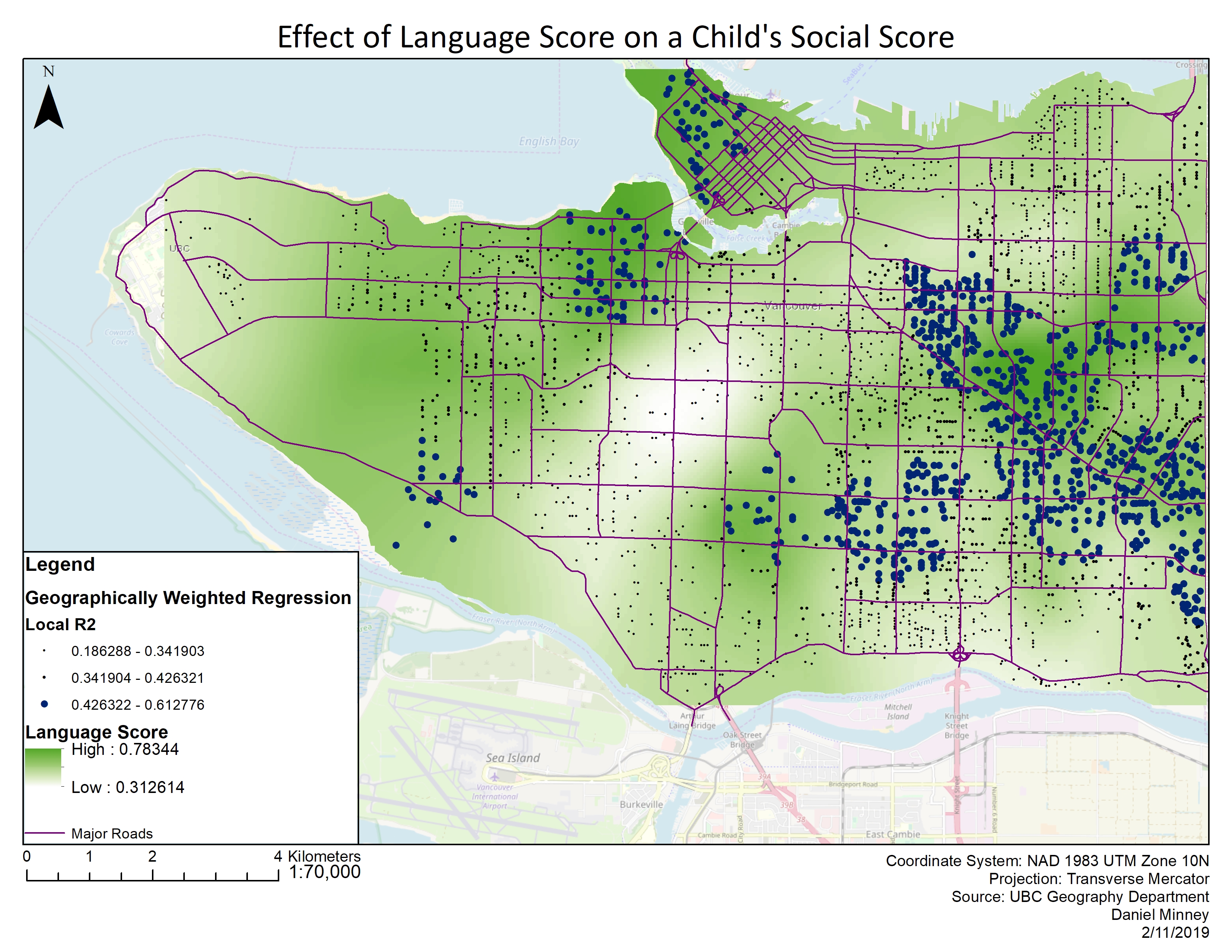
To exercise the use of GWR, the tool was used in ESRI’s ArcMap to explore the relationship between a child’s social score and three variables; income, gender (female or male), and language score. The area of study was Vancouver B.C. in Canada.

The Ordinary Least Squares (OLS) tool is useful because it provides statistics for the three variables chosen. Probability (p) is one of the more useful statistics as it tells which variables are statistically significant. The OLS results show that every variable except for income have a p-value of 0, indicating that they are statistically significant. Income on the other hand has a p-value of 0.10, meaning there is a 10% uncertainty in the data. The r² value from the OLS results were improved upon when using the GWR tool to provide a local r² value.

Income’s effect on a child’s social score, although deemed to be statistically insignificant, still provides some interesting results. East Vancouver particularly contains the lowest scores (most negative results) which indicates that income has a negative impact on the child’s social score. Although no concrete evidence is given, it could be guessed that a lower income has a negative effect because there may be an inability to afford extra-curricular activities, daycare, and other social activities for children. High local r² values also overlay the areas where the lowest negative income values occur, up to -17. Interestingly, in the same areas where income had the lowest values, language and gender both had some of their highest values. Interestingly, in the grouping analysis map produced (Figure 2), most of the West side of Vancouver has a higher than normal income, however, the GWR for income shows that these areas do not have much of an effect at all on a child’s social score.

Gender’s effect on a child’s social score produced interesting results. Negative values reached as low as -17 in the Strathcona/Grandview-Woodland area, however, there are few local r² values higher than 0.42 in these areas, indicating that the model does not predict the actual values all that well. There are many areas where gender had a positive effect on social score’s for children, but these values only go as high as 2.25. While there are areas where being a female has a positive effect on a child’s social score, this effect is less significant than in the areas where there is a negative effect.

The GWR for language score (seen in figure 1) is interesting because there are only positive values, meaning that having a worse language score does not necessarily have a negative effect on a child’s social score. The highest values for language score could be observed in Kitsilano, the West End, and Kensington/Cedar-College, where there are also high local r² values, indicating that the model does a good job in predicting the values.

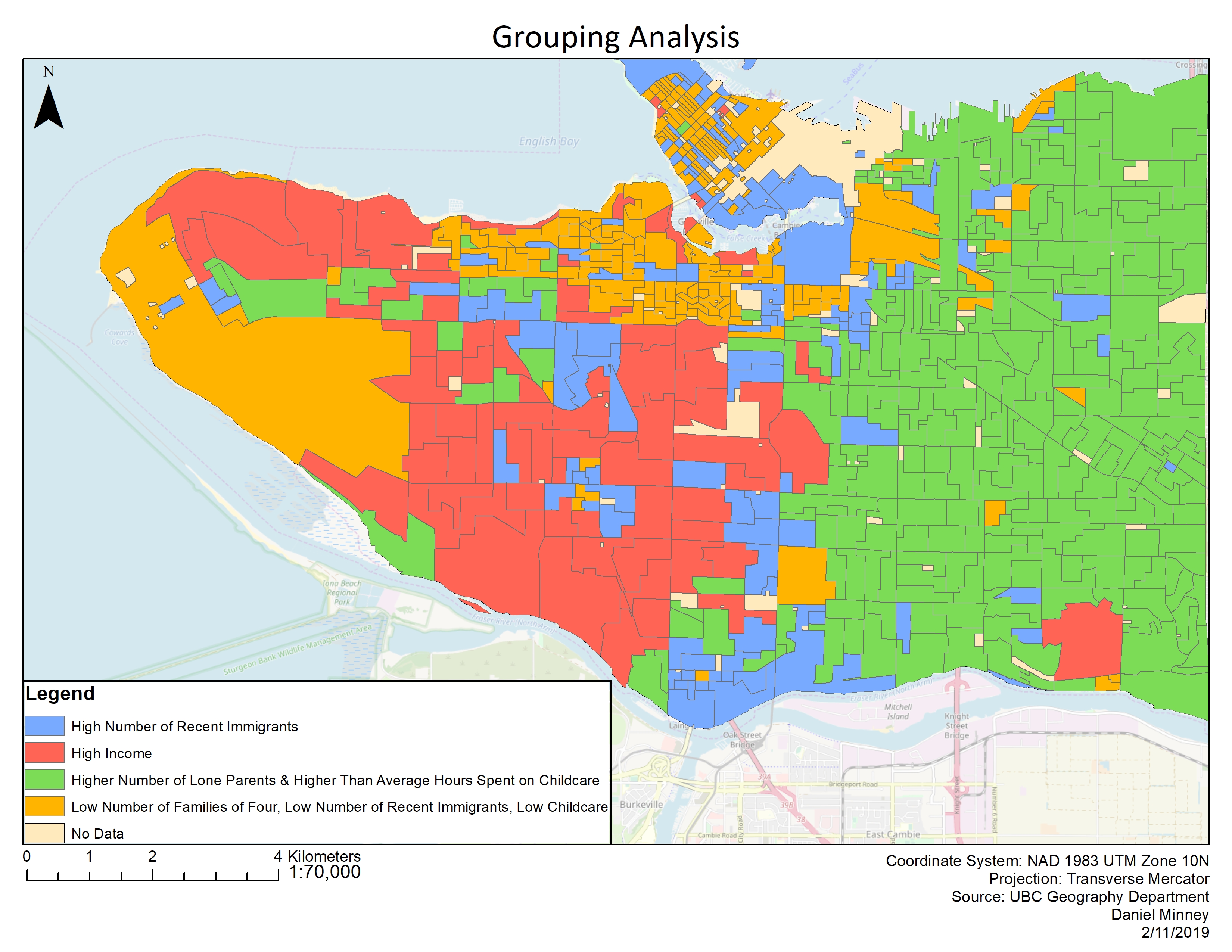
A grouping analysis (seen in figure 2) was performed to aid in understanding the GWR results. By looking at the parallel box plots produced using the grouping analysis tool, arbitrary names were given to each of the four groups. None of the variables for any of the groups existed outside of the upper or lower global whisker, meaning that there are no outliers. East Vancouver is largely dominated by households that have a high number of lone parents and higher than average hours (30 hours) spent on childcare. This would make sense as single parents probably cannot make enough money to afford childcare, and instead spend their own time on it.  The West side of Vancouver was largely dominated by high income areas, as well as some areas with a higher number of recent immigrants. The group containing a low number of families of four, a low number of recent immigrants, and a low number of hours spent on childcare is generally found around the UBC endowment lands which consists of students, as well as Kitsilano and Downtown Vancouver. These areas are generally more expensive and contain smaller homes, so it makes sense that there are less families of four and a lower number of hours spent on childcare.

Geographically Weighted Regression in Other Contexts

Understanding the effects of multiple variables on social scores is just one of the ways to utilize GWR.  A study conducted in 2013 utilized GWR to estimate ground-level PM_2.5 concentrations in the southeastern United States (Hu et al, 2013). A lot of the existing models used global methods for predicting PM_2.5 concentration using satellites and aerosol optical depth (Hu et al, 2013). To add more accuracy to the predictions of PM_2.5 the authors introduced a GWR model to consider local variations (Hu et al, 2013). The results showed that the combination of GWR and aerosol optical depth as well as the other parameters used was able to generate a better model fit, and “achieve a higher accuracy in PM_2.5. The results were as expected, as predicted PM_2.5 values were much higher in urban zones due to factors such as higher car and road density (Hu et al, 2013). Contrasting this were rural and mountainous areas which contained low values for PM_2.5 concentration (Hu et al, 2013). By producing a suitable GWR model, the authors were able to achieve much higher accuracy in predicting PM_2.5 concentration. This use GWR could be used for similar settings such as predicting pollutants from wildfires or other micro-scale meteorology that varies over space.

Another study, conducted in 2012, explored the use of GWR to understand the relation between geographic factors, such as climate, natural resources, or waterways, and how they affected human activities (Yoo,giantelephant6

2). The author noted that OLS, a common regression method, was too limited in describing such spatial patterns and instead opted to use a GWR, as it allows for “coefficients of explanatory variables to differ by locality” in turn incorporating spatial autocorrelation, as well as the idea of Tobler’s first law. The results from the GWR showed that there was indeed a relationship between height and mortality in the Midwest United States, and that as access to water transport increased mortality and decreased stature in the food exporting of the Midwest (Yoo, 2012). GWR was specifically useful in this study as it allowed for local values at the county scale (Yoo, 2012). This study was a good example of how GWR could be used in social and economic research, a topic that is intertwined into geography.

Geographically weighted regression kriging (GWRK) was used by Kumar et al. to enhance the accuracy of typical regression kriging (2012). The study focused on the relationship between soil organic carbon stock (SOC) and various environmental variables which included temperature, precipitation, elevation, slope, geology, and land use (Kumar et al, 2012). The purpose of the study was to compare the two regression methods when estimating SOC stock at 1 metre depth. Suspected to be a result of using local regression values, the GWRK model improved r² values from 0.23 to 0.36.

All the studies cited provide useful examples of how geographically weighted regression was useful in increasing accuracy by producing local values as opposed to using global values for the whole research area. The contexts of these studies are just a few ways that GWR can be used in research. It is likely that with this success GWR will be applied to countless future studies which contain spatial variability.  

Works Cited

Columbia University. (2018). Geographically Weighted Regression. Retrieved from: https://www.mailman.columbia.edu/research/population-health-methods/geographically-weighted-regression

ESRI. (2018). How GWR works. Retrieved from: http://desktop.arcgis.com/en/arcmap/10.3/tools/spatial-statistics-toolbox/how-gwr-regression-works.htm

Fotheringham, A. S., & Oshan, T. M. (2016). Geographically weighted regression and multicollinearity: Dispelling the myth. Journal of Geographical Systems, 18(4), 303-329. doi:10.1007/s10109-016-0239-5

Hu, X., Waller, L. A., Al-Hamdan, M. Z., Crosson, W. L., Estes, S. M., Estes, M. G., . . . Liu, Y. (2013). Estimating ground-level PM2.5 concentrations in the southeastern U.S. using geographically weighted regression. Environmental Research, 121, 1-10. doi:10.1016/j.envres.2012.11.003

Kumar, S., Lal, R., & Liu, D. (2012). A geographically weighted regression kriging approach for mapping soil organic carbon stock. Geoderma, 189-190, 627-634. doi:10.1016/j.geoderma.2012.05.022

Yoo, D. (2012). Height and death in the antebellum united states: A view through the lens of geographically weighted regression. Economics and Human Biology, 10(1), 43-53. doi:10.1016/j.ehb.2011.09.006

Figures