For prioritization of restoration sites in Hope, first I created 2 criteria, each including sub-criterions, primarily using Lane et al. (2008) paper and considering data available. The first criteria focuses on prioritizing sites with high probability of restoration success and the second concentrates on prioritization of sites that would have highest restoration efficiency. After creating separate maps for each sub-criterion, I conducted a Boolean Multi Criteria Evaluation (MCE) for criterion one due to categorical nature of my data. Then, I reclassified the slope layer I created (from a contour layer) appropriately for criterion two (see flowcharts here). Here are my criteria including their logic and data sources:
1) Prioritizing sites with high probability of restoration success
Restoration is more likely to be successful in areas that are not exposed to threats or stressors such as human disturbances. Therefore, areas with the least threats / stressors were ranked highest and used for mapping highest priority sites. The report (Lane et al., 2008) provides rankings for each of the below sub-criteria, which used to map the highest ranked conditions. Each sub-criterion fits one of the categories of ‘constraint’ or ‘factor’ for the Multi Criteria Evaluation (MCE). The constraints are taken out of the final map and the factors are used to map the sites.
Factors:
- Areas with minimal human disturbance
I omitted areas that are highly impervious for this section since a high percentage of impervious cover is often associated with excess heat, trampling, salt, sand, snow damage etc. I erased categories of ‘poor’ and ‘very poor’ from soil drainage data. Data: Soil Drainage shape file from HectaresBC
- Surface Material
Restoration is only possible in sites with organic or mineral soil (no rock). Therefore, I will identify and add these areas to the map. Data: Surface Material from HectaresBC
Constraints:
- Salt / spray runoff
Salt spray and/or run off could threaten plant survival. Ranks of threat of salt spray are based on proximity to different road types. High traffic roads (4 lane or more) were buffered for 600 feet in either side and low/medium traffic roads (3 lane or less) were buffered for 120 feet for least threat scenario. Data: Roads in TRIM
- Railroad
Areas that are under ‘active’ railroad corridors will be subjected to maintenance; thus are not ideal for restoration. To separate ‘active’ railroads for the project, I erased ‘abandoned rail lines’ from the layer. Then, buffered ‘active’ railroads for 300 feet for lowest threat/stressor. Data: Rail lines in TRIM
- Utilities, buildings, industrial area etc.
Similarly, areas in vicinity of utilities, building etc. are subject to maintenance and human disturbance. Therefore, like railroads, utilities were buffered for 300 feet. Although for this sub-criterion I went through all the different classes and types of utilities and industries and found one type, ‘abandoned site’ under the class ‘extraction site’, that could undergo restoration since it’s not active anymore. Therefore, I omitted the buffers of these sites from the map. Additionally, I found this data as lines so I had to change some classes to polygons for buffering while I kept the appropriate classes as lines. Data: Utilities in TRIM
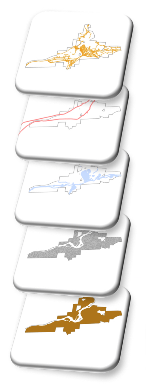
The figure below shows all my layers of constraints and factors before analysis.
2) Prioritizing restoration efficiency
Some polygons require less resources to implement and maintain restoration. These sites were prioritized and determined by slope of the site.
- Site slope
Restoration on steep slopes typically requires more resources for activities such as site preparation. Additionally, on steeper slopes the use of tractors and other machinery is usually difficult. Therefore, flatter slopes are prioritized in this project using reclassify tool. I identified slopes of higher than 10% with ‘NoData’ and reclassified slopes of 0-10% into for equal breaks for analysis. Since the availableDigital Elevation Models (DEM) had large pixel sizes, before reclassification, I created a TIN layer using contours, water lines and roads. I used ‘TIN to Raster’ tool to create a DEM following a Slope layer from DEM, which I used for this criteria. Data: Contours from GeoGratis
In the end, the criterion two layer was converted to vector data (using Raster to Polygon tool) and intersected with criterion one for further analysis and discussion.