In this lab we conducted an assessment of land use change around Edmonton, Alberta between 1966 and 1976. I focused my study on urban land use change to measure urban expansion over 10 years.

The amount of urban built-up areas in Alberta increased almost tri-fold over these ten years from 19,596 hectares in 1966 to 54995 hectares in 1976. However, the growth was seen not only in the expansion of the city core but also in an increase in number and size of disjunct areas. The urban areas were built on what was previously cropland, pastures and productive woodland. Further rapid urban growth is expected and an effective land use management plan is necessary to manage urban expansion with minimal costs to the surrounding environment.

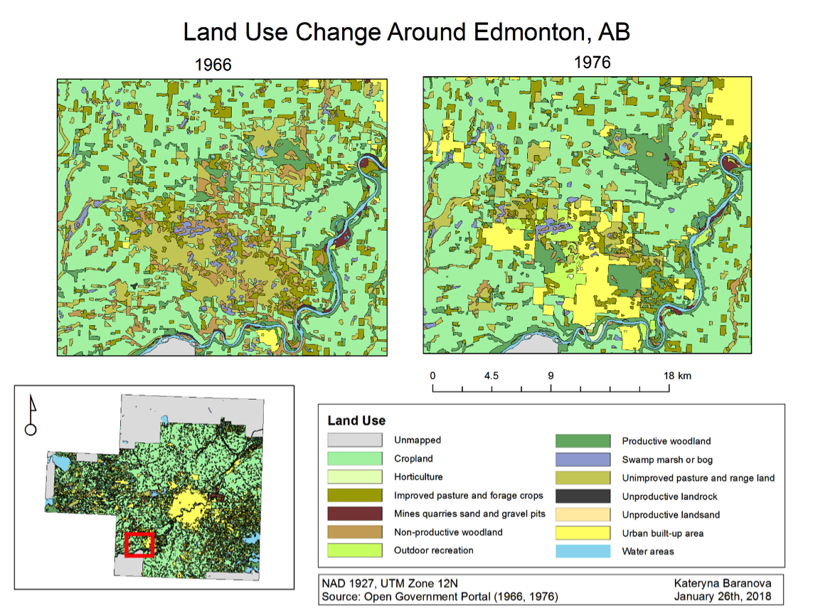
The data used for analysis in this report was retrieved from the Open Government Portal. The analysis uses CLUMP (Canada Land Use Monitoring Program) data for Edmonton, Alberta in the years of 1966 and 1976. It includes 14 land use classes that were sorted based on air photo interpretation, field surveys and census information. ArcGIS was used to produce two maps depicting various land use classes in 1966 and 1976 (Map 1) and then looked closer at urbanization of the urban core (Map 2) and the peripheral land (Map 3). It can instantly be seen (Map 1) that both the core and peripheral areas experienced rapid urban growth over 10 years. The built-up areas increased in number and size taking over other land uses. If we look at the core urban area of Edmonton (Map 2) we can see that it grew significantly, taking over what was cropland and pasture in 1966 and replacing. As mentioned above, the amount of disjunct areas around the core also increased with urbanization moving further away from the center. If we look at the change in one of such areas (Map 3) we can see that urbanization replaced pastures, cropland and marshes.

Through using FragStat for analysis, the total area of the built-up areas class increased by 35399 hectares with the total core area increasing by 22560 hectares. Built-up areas almost triple and came to occupy 8.5407% of the study area in 1976 compared to only 3.0413% in 1966. The number of disjunct urban areas also increased from 88 to 384 within ten years indicating a shift away from the core urban area (Table 1). Although the number of patches increased greatly for urban areas from 133 to 417 the number of patches for the whole landscape decreased by 209 therefore indicating a loss in landscape diversity most likely caused by urbanization (Table 2).

To analyze where the increase in the built-up areas came from in 1976 we created a transition matrix (Table 3). We can see that built-up areas from 1966 contributed only 35.63% of the total 1976 area. Most of the 1976 built-up areas came from cropland 38.88% followed by unimproved pastures and range land 13.51% and productive woodland 5.00%. Figure 2 you can see the complete breakdown of what land use classes in 1966 have been converted to built up areas in 1976. Can conversion of productive land to urban areas can be problematic in the long term therefore it is important to understand where urban growth comes from.

In figure 1 we can see the land use total areas by classes between 1966 and 1976. We can see that most land use classes decrease in area that they occupy and the two most significant increases can be attributed to built up areas and productive woodland. The latter can be explained by the maturation of unproductive forest land from 1966 to 1976.

Table 1: Changes in class level metrics for land use in Edmonton, Alberta between 1966 and 1976.

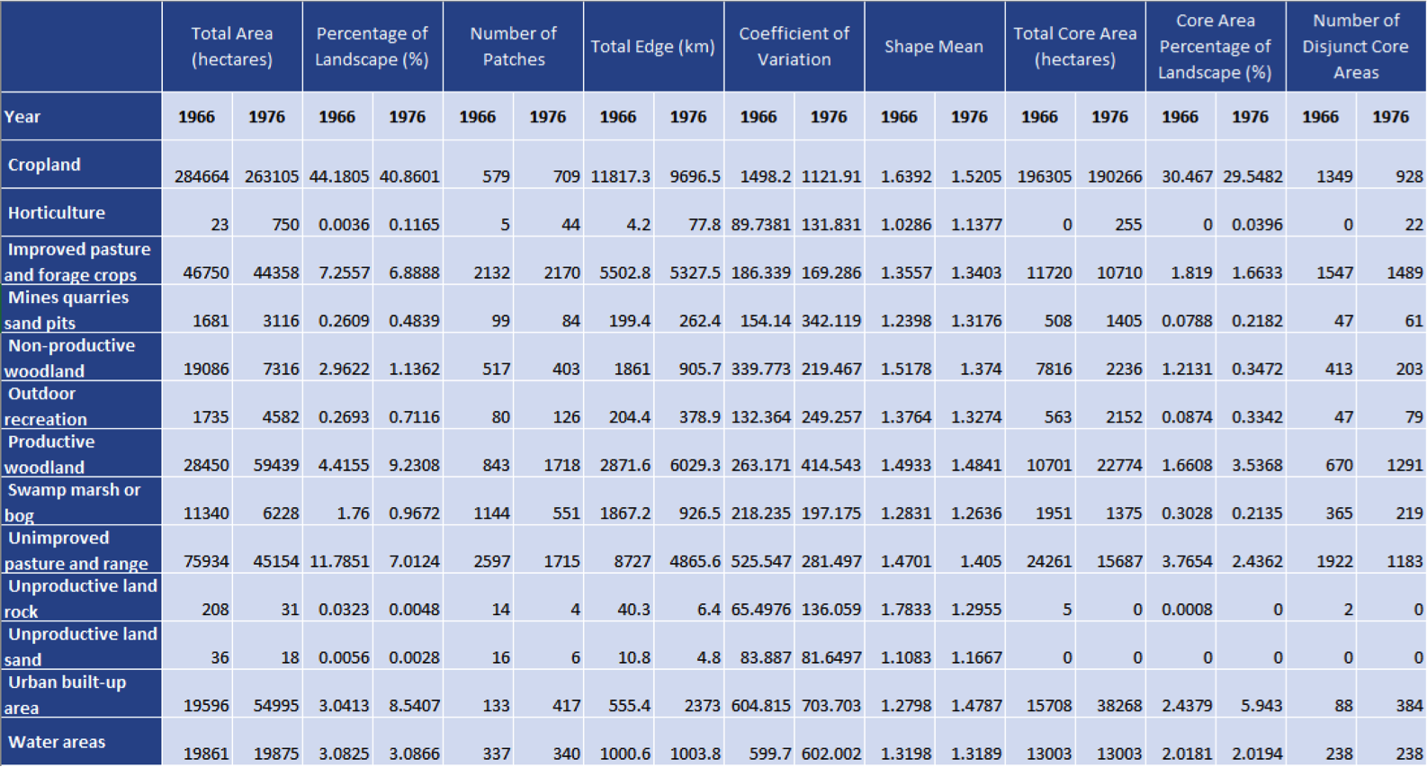
Table 2: Changes in landscape level metrics for land use in Edmonton, Alberta between 1966 and 1976.

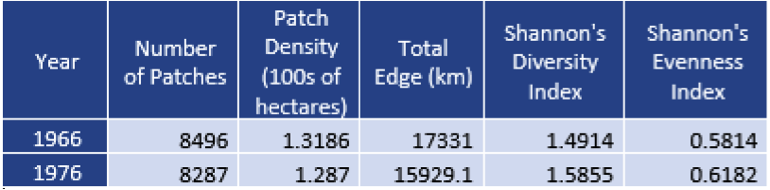
Table 3: Transition matrix depicting where the change in land use in 1976 came from.

Table 4: Description of class and landscape metrics used.

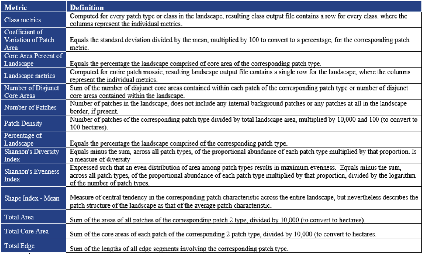
Figure 1: Total areas of land use classes in 1966 and 1976.

Figure 2: Land use class change to urban built up in 1976.

Map 1: Land use change between 1966 and 1976 in Edmonton, AB.

Map 2: Land use change in the core urban center of Edmonton, AB between 1966 and 1976.

Map 3: Land use change in the peripheral urban area in Edmonton, AB between 1966 and 1976.

References

Open Government Portal. n.d. Edmonton CLUMP 1966, 1976. Retrieved from

http://open.canada.ca/data/en/dataset?organization=nrcan-rncan

Kevin McGarigal. 2015. Fragstats Help. Retrieved from

http://www.umass.edu/landeco/research/fragstats/documents/fragstats.help.4.2.p

The below map gives a hot spot distribution of heart disease rates by county in the southern United States. The data for this map was taken from CDC Wonder for the year 2016. The total deaths from heart disease were divided by the total population of the county to find the heart disease rate and normalize the data. Also a spatial weights matrix was created using the 8 nearest neighbors to run the hot spot analysis. Since this is a big dataset, and before zeroing in on 2016 I looked at years 1999 to 2016, models were created in Modelbuilder to process all of the data. The first model was designed to separate the data into 18 yearly classes and process it year by year. The second model used a hot spot analysis tool to define statistically significant hot and cold spots with confidence levels of 90%, 95% and 99%.

By looking at the results of the hot spot distribution we can immediately identify that Oklahoma has the highest concentration of heart disease cases out of all the other southern United States. The east coast and Texas have some of the lower concentrations. Further data and analysis is needed in order to determine the causes of such spatial variations of heart disease rates. Perhaps the concentration of hot spots in Oklahoma could be due to older population, poverty, unhealthy diets, poor air quality, higher caffeine consumption, or even genetically predisposed population. It could also be due to infrastructural distributions and by this I mean a higher concentration of nursing homes and heart disease centers. Any or all of these factors could play a role in determining the patterns, however that information was not available to us for the purposes of this assignment. Overall Oklahoma seems like a problematic state in terms of heart disease fatalities and I would suggest moving to Maryland which seems to be the less troubled according to this map.