Lab 1: Spatial stats using Modelbuilder tutorial
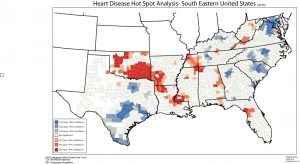
Lab 1 involved an introduction to model building. Data was used from the CDC Wonder Data in order to create animated hotspot maps of hearth disease in the southern united states by county. A model was formed which allowed for18 individual feature classes to be created which were then animated. This was then produced into the final product which can be seen below.
Lab 2: Exploring Fragstats
In lab 2 we envisioned ourselves as environmental consultants hired by the city council of Edmonton in order to produce a report demonstrating changes in the landscape metrics of the surrounding area. The goal of this lab was to observe how landscape change had occurred in Alberta between 1966 and 1976. Moreover, additional emphasis was placed on landscape metrics. In order to accomplish this goal we implored the use of Fragstats (a nifty tool which allows for complex statistical analysis of TIF files). We used fragstats in order to calculate a series of landscape metrics such as edge depth,area,percentage of landscape and shape index. In total 14 different landscape and class metrics were used. From there we used these results in order to create a transition matrix to show how the landscape changed. This involved the creation of rasters and a series of joins and relates.Lastly we created a pivot table in order to show in a simple to read way the results of the landscape change. All of these results can be viewed below.
Land Use in Edmonton Alberta- Report
Land Use in Edmonton Alberta-Map
Lab 3: Introduction to Geographically Weighted Regression.
Lab 3 dealt with issues related to geographically weighted regression. Within Vancouver variables such as language score, gender, and income were examined for their impact regarding childhood development. Furthermore, these variables were then examined spatially across the city as to observe possible patterns.
Below is a summary of GWR and two maps from the final results which depict childhood language score and neighborhood income values. Geographically weighted regression (GWR) is a class of linear regression which is applied in order to examine local relationships. The most notable function of GWR is the modeling of the relationship between dependent and explanatory variables based on location. Unlike global models, a local model such as GWR is able to apply the explanatory and dependent variables on a case by case basis based upon locale. As such, GWR is able to model how variation occurs across an area of study. GWR as a form of spatial regression has many similarities to ordinary least squares models (OLS). In simplest terms OLS models are used to predict the unknown values in linear regression models. GWR requires two variables, respectively being the dependent and the explanatory variable. Explanatory variables though similar to independent variables are distinct due to outside variables effecting them. In other terms, explanatory variables are not completely independent from the effects of other variables, though they are not to be mistaken for a dependent variable. Additionally, dependent variables are those which respond to the effects of the explanatory variable. An example of this relationship would be looking at how the effect of income by neighborhood across an entire city effects crime. Returning to the previously mentioned OLS, a GWR is able to model a separate OLS for every point (or location) being examined. Another essential component of GWR is bandwidth. Bandwidth refers to the parameters related to kernel type, distance and number of neighbors. Important to note is that when the number of neighbors’ parameter exceeds 1000, then only the nearest 1000 are incorporated in each equation (“Geographically Weighted Regression,”2016). Furthermore, GWR is restricted when applied to small data sets and when used with multipoint data. (“Geographically Weighted Regression,”2016) Due to the regression technique it is also important to consider the data being used. When using GWR it is crucial to avoid binary data that is data with only two possible outcomes such as 0 or 1. In turn GWR is only suitable for data which includes a variety of numeric values.
Vancouver Neighbourhood Income Values-Standard Deviation
Childhood Language Score-Standard Deviation
Lab 4: Introduction to CrimeStat
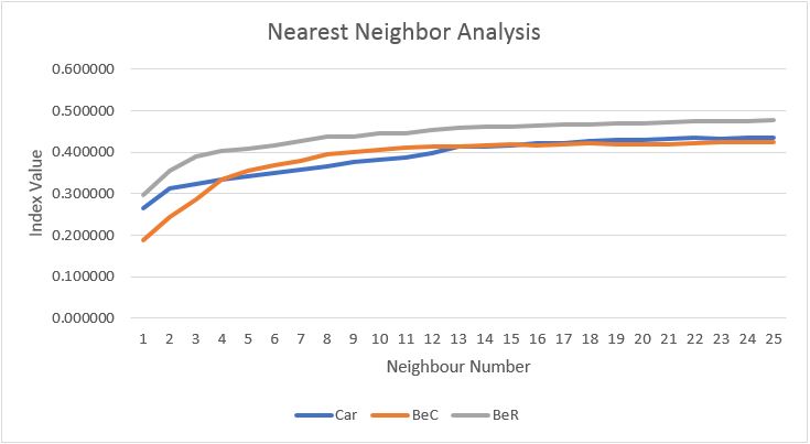
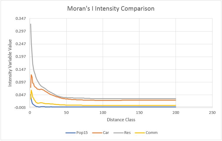
Lab four was a return to crime statistics which had been examined before in GEOB 370. Approaches taken in this lab extended on prior knowledge and were based in more advanced techniques. Moreover, the program Crime Stat was introduced in order to measure the statistical importance of results. Analysis revolved around nearest neighbor, fuzzy mode, hierarchical clustering, correlograms and risk adjusted models. Additionally, a knox index was run in order to test of temporal importance and to see if any patterns occurred throughout space and time. Two kernel density maps were as well produced which are attached below along with an example of the knox index.
Knox Index: Interaction of Space and Time

   Sample size ...........:  2152

    Measurement type ......:  Direct

    Input units .... ......:  Meters

    Time units ............:  Hours

    Simulation runs .......:  19

    Start time ............:  09:46:37 AM, 03/09/2018


    "Close" time ........:            6.00000 hours

    "Close" distance ....:         5000.00000 m


                         | Close in space(1)  | Not close in space(0) |

    ---------------------+--------------------+-----------------------+-----------------

    Close in time(1)     |             456592 |               1421931 |      1878523

    Not close in time(0) |             111845 |                324108 |       435953

    ---------------------+--------------------+-----------------------+-----------------

                         |             568437 |               1746039 |      2314476


    Expected:

                         | Close in space(1)  | Not close in space(0) |

    ---------------------+--------------------+-----------------------+-----------------

    Close in time(1)     |       461366.62404 |         1417156.37596 | 1878523.00000

    Not close in time(0) |       107070.37596 |          328882.62404 | 435953.00000

    ---------------------+--------------------+-----------------------+-----------------

                         |       568437.00000 |         1746039.00000 | 2314476.00000


    Chi-square ..........:          347.73143

    P value of Chi-square:            0.00010


    End time ..............:  09:46:38 AM, 03/09/2018


    Distribution of simulated index (percentile):

    Percentile      Chi-square

    ---------- ---------------

          min         0.00007

           0.5         0.00007

           1.0         0.00007

           2.5         0.00007

           5.0         0.00007

          10.0         0.01274

          90.0         1.79751

          95.0         2.42568

          97.5         2.42568

          99.0         2.42568

          99.5         2.42568

           max         2.42568