Streamflow regime classification
The classification result of the test data (30% of the 1448 selected stations) is showed as a confusion matrix and statistics by class in Table 1. The overall accuracy of the model created by XGB is 88.9% while the No Information Rate (NIR) is 66.1% (the accuracy if all the records were classified as the majority class, the nival class in this case). The p-value for the hypothesis that overall accuracy is greater than NIR is 2.2-16, which indicates the model is statistically robust. In Table 1b, the balanced accuracy for each class is ranging from 81.6% to 99.5%. The model performed relatively poorly for the nival-hybrid class. 20% (5 out of 25) of the observed nival-hybrid class was incorrectly classified as nival. This could relate to the great similarities between the nival-hybrid regime and nival regime, which can be observed in Fig 1 (Coquihalla vs. Redfish).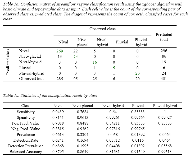
The top 10 most important variables (see Appendix 1 for descriptions of variables) that contributed to the classification, based on the gain in information from a single split of data, are showed in Fig. 2. The easting of the UTM coordinate of the station is the most important feature dominating the classification. It is followed by the autumn mean temperature (tave_at), mean annual summer precipitation (msp), temperature difference between the mean warmest and coldest month temperature (td), and days above 18oC in spring (dd18_sp). In fact, both easting and td are pointed to continentality. Easting directly relates to the distance from the coast, and inland areas tend to have higher td than those coastal areas have. Therefore, continentality plays an essential role in streamflow regime classification, which in turn matches the spatial distribution of regimes described by Eaton & Moore (2010). For example, nival regimes occur in the interior plateau and mountain regions while pluvial regimes are found primarily in coastal areas. However, there may not exist a linear relation between quantified continentality (e.g., td) and streamflow, so it is difficult to detect such relation using traditional linear regression methods. On the other hand, tree-based methods have the advantage to discover non-linear relations in a understandable way, by spliting the data. Altough the actuall trees produced by tree-ensemble algorithms such as XGB are not interpretable (there are thoudsands of trees),
insights on the underlying processes can still be shed through the importance of variables.
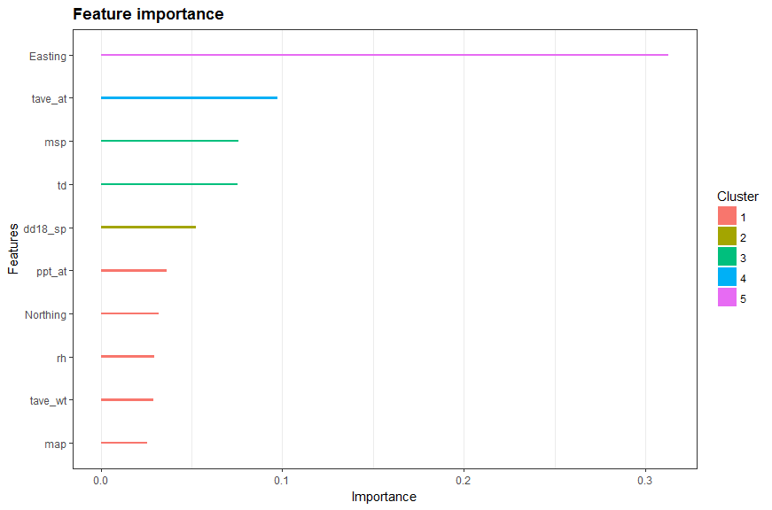
Figure 2 The top 10 most important input variables for streamflow regime classification determined by the xgboost algorithm
The spatial distribution of the correctly/incorrectly classified regimes is plotted in Fig 3. Red dots represent locations where the streamflow regimes were incorrectly classified. The distribution of red dots does not exhibit obvious clustering. This could imply the model generated by XGB might be not biased by the unevenly distributed gauging locations.
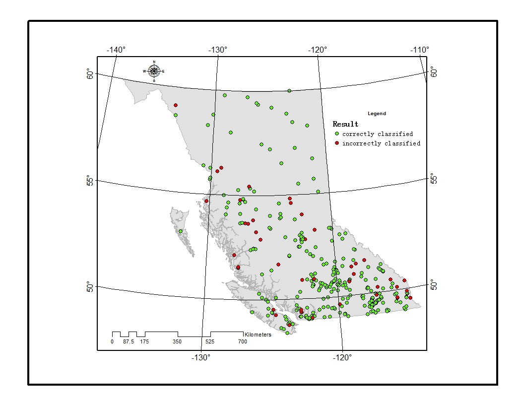
Figure 3 The spatial distribution of the classification result. Green dots represent locations that the streamflow regimes were correctly classified, while red dots represent locations with incorrectly classified results.
Mean annual discharge prediction
The attempt of empirically predicting the mean annual discharge using XGB was not as successful as the regime classification. The predictive power of the model created is limited. The R2 value of the relation between observation and prediction is 0.72 in Fig 4a. The frequency distribution of the absolute value of percent error in predictions for the 399 test catchments is displayed in Fig 5a. The 1st quantile, median and 3rd quantile of the absolute percent error are 19.3%, 45.9% and 118%, respectively. However, there exists two outliers up to thousands times over-predicting the observed value.
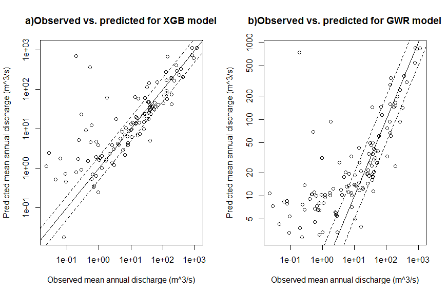
Figure 4. Comparison of the performances of the XGB and GWR models. In each graph, the observed mean annual discharges (m3/s) for the 399 test catchments are plotted against predicted values. The solid line indicates perfect prediction, and the dashed lines represent +/- 30% error.
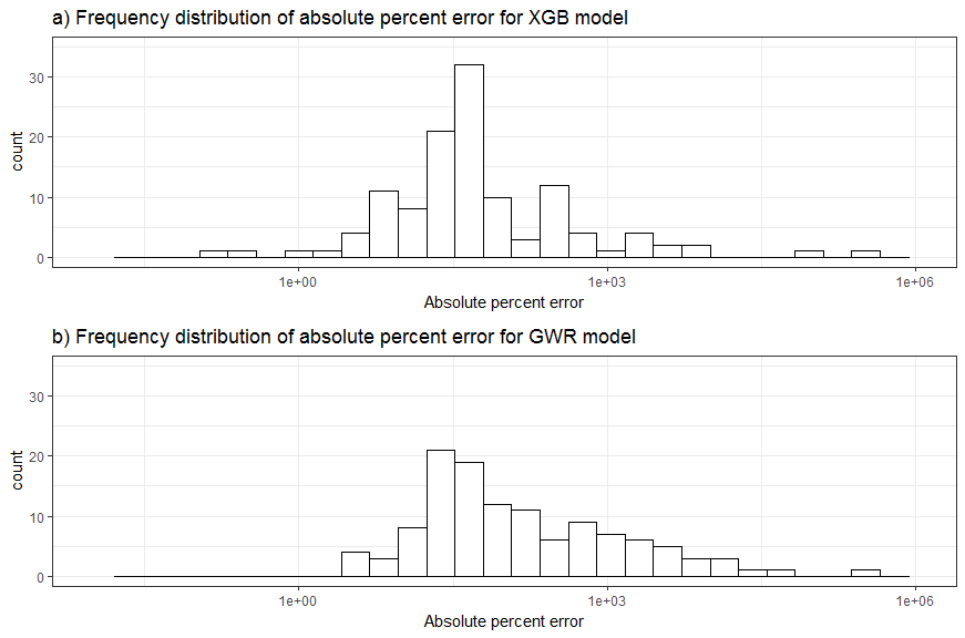
Figure 5. Frequency distributions of the absolute value of percent error for the two models. Note that the percent errors exhibit different orders of magnitude, thus the errors are in absolute value form in order to use log scale.
Although the performance of the model is moderate, the feature importance determined by XGB (Fig. 6) is still informative. The top 3 most important variables: basin stream magnitude (L_MAG), drainage area in m2 (DRAIN_M2), and mean cumulated annual precipitation over the entire basin in mm (CCMLTVPRCP) have strong correlations to the observed mean annual discharge (Fig. 7). For comparison purpose, the Geographically Weighted Regression (GWR) technique (Brunsdon et al., 2002) was used to model the relationship between these three variables to the mean annual discharge. The GWR has advantages over the traditional Ordinary Least Square (OLS) regression as it allows the relation varies over space and has the ability to provide local error measurements for spatial variation diagnosis. The overall R2 value of the GWR model is 0.81 (Fig. 4b), which is higher than the XGB model. However, its frequency distribution of absolute percent error (Fig. 5b) indicates that its performance is in turn inferior than the XGB model. This is probably due to a known effect that the model is biased by the “nature of the stream gauging network”. Stream gauges tend to be concentrated in areas with higher population and at lower portions (in terms of elevation) of the stream network, resulting in nonrepresentive sampling of basins (Trubilowicz et al., 2013). The local R2 map of the GWR model (Fig. 8) exhibit such effect. Low R2 values are clustered at populated regions where the gauges are densely distributed, including Vancouver Island and lower main land (southwest), Okanagan and Kootenay regions (southeast).
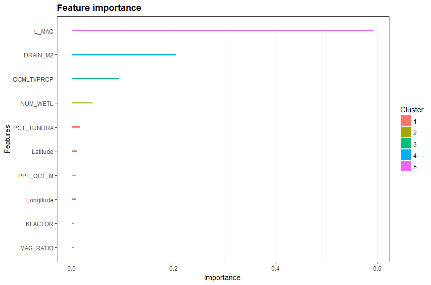
Figure 6. The top 10 most important input variables for mean annual discharge prediction determined by the xgboost algorithm. Note that all the input variables, except latitude and longitude, are from the EAUBC Rivers dataset.
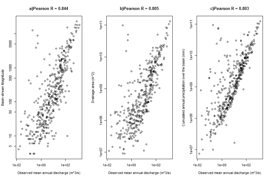
Figure 7. Correlations between the most three important variables determined by XGB and the observed value. Note that both axes are in log scale for visualization purpose. The Pearson correlations (shown in the figure) without log transformation are actually greater than those (not shown) after log transformation.
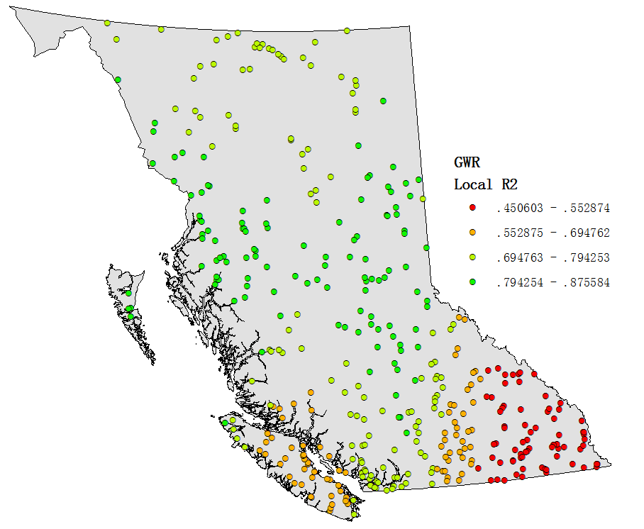
Figure 8. The local R2 map of the GWR model. Low values exhibit clustering at populated regions.
Besides the bias from the gauging locations, it can be observed that there exists large systematic error when the observed values are smaller than 1 m3/s in Fig. 4. Both models tend to significantly over-predict for catchments that have low flows. This could be caused by missing important variables or error in the input data. Further studies are required to investigate the sources of this error.