1. Chris Conlon’s IO course
2. Paul Goldsmith Pinkham’s Applied methods course
3. Gary King’s quantitative social science methods lectures.
4. Florian Oswald’s course on computational methods.
5. Gilbert Strang’s video lectures on linear algebra.
6. Recordings of past Chamberlain lectures on econometrics.
7. Corporate income tax.
8. Adam Kucharski’s lecture on contagion.
9. Ed Rubins DAG slides.
10. Grant McDermott’s Data Science for Economists.

The ordering above is basically random.

One thing Stata users miss in R is an easy way to do the following operation.

foreach x of varlist lnw age asq bmi hispanic black other asian schooling cohab married divorced //
separated age_cl unsafe llength reg asq_cl appearance_cl provider_second asian_cl black_cl hispanic_cl // othrace_cl hot massage_cl {
egen mean ‘x’=mean(‘x’), by(id)
_
gen demean ‘x’=‘x’ – mean ‘x’

drop mean*
}

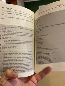
This example is taken from Scott Cunningham’s super book, Causal Inference: the Mixtape. In the lower right of the picture you can see the demeaned variables being created one by one. So how does one perform an operation to create a large number of variables?  My preferred method is to take advantage of the .SD functionality in data.table. Create a character vector like this: myvars <- c(“lnw”,”age”) with all the variables you want.

demean <- function(x) x- mean(x)
DM <- DT[,lapply(.SD,demean),by=id,.SDcols=myvars]

Note how general this is since demean could be replaced a great number of other operations.

Also note that DM won’t have all the “demean_lnw” variables. The demeaned variables in DM keep their names from before. i think that’s a plus for various reasons.  if you want the variable names, Grant McDermott showed me that you just use the := as follows:

DT[, paste0(myvars, ‘_demean’) := lapply(.SD,demean), .SDcols=myvars, by=id]

However suppose you want to do something more along the lines of a foreach loop. then the following is more like the Stata code in terms of style and effects:

for(i in 1:length(myvars)) {
DT <- within(DT,{assign(paste0(“demean_”,myvars[i]),get(myvars[i])-ave(get(myvars[i]),id))})
}

The crucial function to learn is assign. Its first argument is string to be used as the name of the variable you’ll create and the second argument is the value you want to assign to that variabel. The get function just converts a string like “age” into an R object age.

Seeing today that more and more people are considering giving up on Stata based on their horrible pricing policies, I offer this collection of very frequently used Stata commands and how to do roughly the same thing using R. But not with dplyr and pipes and all that.  This how-to uses only base R, data.table, and fixest.

1. Insheet, import a CSV file
   • R data.table::fread()
   • R advantages: faster for huge files, usually guesses what you want, can work with files from internet or zipped files
2. Replace y if x something
   • DT[, y := x] #initialize a new variable equal to existing variable x in the datatable called DT
   • DT[x>5, y := 5]  # now censor the y version
   • DT[is.na(x), y := 0] # now code the missing x to be 0s in the y variable
3. Rename variables:
   • setnames(DT,old=c(“blah”,”blah_blah”), new=c(“x1″,”x2”)) renames blah to be x1 and blah_blah to be x2. all other variables keep their names.
   • The old variables can be just a range of columns as in old=5:12
4. gsort x -y: setorder(DT,x,-y)
5. Merge
   • DT1 <- merge(DT1,DT2,by=c(“id1″,”id2”),all.x=TRUE) is like if in Stata merge 1:1 id1 id2 using DT2.dta followed by drop if _merge==2
   • if you don’t want to drop anything, use all =TRUE
   • R’s version of merge allows for the id vars to have different names in DT1 and DT2, e.g. suppose your country code is “iso” in DT1 but “iso3” in DT2. similarly “year’ and “yr”. then you write DT1 <- merge(DT1,DT2,by.x=c(“iso”,”year”),by.y=c(“iso_o’,”yr”),all.x=TRUE)
6. Collapse and egen: these are the two commands i use the most and i still call them by their Stata names
   • collapse (mean) x_i = x_it, by(year) would be DTc <- DT[,.(x_i =mean(x_it)),by=year]
   • egen x_i = mean(x_it), by(year) would be DT[,x_i := mean(x_it),by=year]
   • if there are more than one by variables, both commands use .(iso,year)
   • Note1: the collapse must be “sent” to a data.table. If we don’t need the original DT, we could <- it to DT.
   • Note 2 The “:=” is essential in the egen-equivalent. It does something called “modification by reference”
7. Reshape long or wide. While the syntax of reshape is often said to be hard to remember, data.table’s melt and dcast are even harder to keep straight but they are very flexible and powerful functions.
   • reshape long MFN_, i(iso_d year) j(product) string
   • DTl <-melt(DTw,id.vars=c(“iso_d”,”year”),measure=patterns(“^MFN_”),value.name=”MFN”,variable.factor = FALSE)
     DTl[,product := substr(variable,5,nchar(variable))] # extract code
     DTl[,variable := NULL] # we don’t need “variable” anymore
   • the reshape wide is done with dcast()
   • DTw2 <- dcast(DTl,iso_d+year~product,value.var = “MFN”) # the variables in the formula before the “~” are id vars that stay as rows. the variable to the right of “~” is the column variable.
   • in contrast to “reshape wide” dcast on a single value.var will name the columns after the “product” variable
8. Drop/keep conditionally: In data.table you drop by selectively keeping.
   • Drop if x==. | y==0
   • DT <- DT[!is.na(x) & y!=0]
9. Save/use: The first thing you need to do when getting started is go to Rstudio’s preferences settings and make sure you NEVER save or restore the workspace in .Rdata.  Furthermore, you should make a practice of restarting the R session fairly regularly.  But that’s just an aside. I save data as RDS forms which is automatically compressed.
   • use  is done by DT <-readRDS(“path_to_file/file.rds”)
   • save is saveRDS(DT,”path_to_file/file.rds”)
10. reghdfe (AKA AKM). The pioneer was Simon Gaure’s excellent lfe::felm(). But for most purposes you should probably use Berge’s fixest::feols(). Not only is it faster, but it will make it easier to transition to various GLM in item 11.
    • res.ols <- fixest::feols(log(y) ~ educ + age+ I(age^2) | worker_id +firm_id,data=DT)
    • summary(res.ols)
11. ppmlhdfe res.ppml <- fixest::fepois(y~educ+age +I(age^2) | worker_id +firm_id,data=DT)
    Setting combine.quick to FALSE is useful  when you specificy interactive fixed effects (fixest has a great notation for this) want to do something later with the Fixed effects and need to know which country-year FE they correspond to. fepois is a special case of feglm, which can be used for non-poisson specifications.
12. esttab (LaTeX table of regression results)  There are many options for latex tables in the R world with Stargazer probably the best known but I have found the built in etable() function to be quite adequate fixest::etable(res.ols,res.ppml,sdBelow = TRUE,digits=3,fitstat=~sq.cor+pr2,
    tex=TRUE,file=”Tables/AKM_regs.tex”,signifCode = “letters”,cluster=”worker_id”,replace = TRUE)