Data
The data used in this analysis was collected from a number of Norwegian government agencies and institutions (Table 1).
Table 1: Data overview
| Data | Data owner | Link to data distributer | Format | Areal and temporal scale | Notes | |
| Variables for statistical analysis | ||||||
| Difficulty sleeping | NOVA (Oslo Metropolitan University) | Norwegian Institute of Public Health | xls | City district, 2021 | Percent of youth (age 13-16) reporting they have had difficulty sleeping the past week. | |
| Screen time, more than 4 hours per day | NOVA (Oslo Metropolitan University) | Norwegian Institute of Public Health | xls | City district, 2021 | Percent of youth (age 13-16) reporting they usually spend 4 hours or more using screens after school hours. | |
| Pleased with neighborhood | NOVA (Oslo Metropolitan University) | Norwegian Institute of Public Health | xls | City district, 2021 | Percent of youth (age 13-16) reporting they are ‘pleased’ and ‘somewhat pleased’ with their local neighborhood | |
| Children of single parents | Norwegian Labour and Welfare Administration | Norwegian Institute of Public Health | xls | City district, 2020 | Percent of children (aged 0-17) where 1 and not 2 parents receives child support (all parents do regardless of income, in Norway). | |
| Households with persistent low income | Statistics Norway | Norwegian Institute of Public Health | xls | City district, 2017-2019 | Percent of households with persistent low income (more than 3 years), defined by European Union standards. | |
| Households with low income | Statistics Norway | Oslo Municipality | xls | City sub-district, 2019 | Percent of households with low income, defined by European Union standards. | |
| Crowded households | Statistics Norway | Norwegian Institute of Public Health | xls | City district, 2020 | Percent of people living in residence where 1) fewer rooms than people, and 2) less than 25m2 per person. | |
| Wellbeing at school | NOVA (Oslo Metropolitan University) | Norwegian Institute of Public Health | xls | City district, 2020/2021 school year | Percent of youth (age 13-16) reporting high level of wellbeing at school. | |
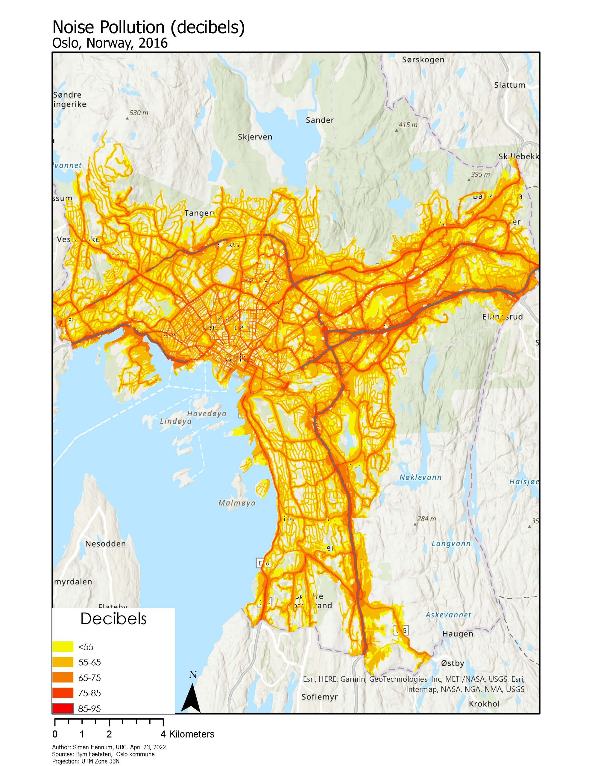
| Noise pollution | Agency for Urban Environment, Oslo Municipality | Distributed via email | Shapefile | Oslo municipality, 2016 | Polygons with attributes in decibel ranges. | |
| Spatial data | ||||||
| Basic Statistical Unit (grunnkrets) | Norwegian Mapping Authority | Geonorge | Shapefile | Oslo Municipality | n=589 | |
| City sub-district (delbydel) | Agency for Planning and Building Services, Oslo Municipality | Distributed via email | Shapefile | Oslo Municipality | n=94 | |
| City district (bydel) | Agency for Planning and Building Services, Oslo Municipality | Distributed via email | Shapefile | Oslo Municipality | n=15 | |
| Shoreline | Norwegian Mapping Authority | Geonorge | Shapefile | Oslo Municipality | Used to clip areal units to shoreline | |
| Land use | Norwegian Mapping Authority | Geonorge | .shp | Oslo Municipality | Noise levels along county and state roads (red > 65dB), yellow = >55dB | |
| Aboveground roads >70km/, trams, railways, subways | Open Street Map | overpass-turbo | GeoJSON | Oslo Municipality | Exclude subterranean features | |
The neighborhood and socioeconomic variables selected for an initial exploratory regression analysis were included on the basis that previous research indicate that they are correlated (Bøe et al., 2012; Sivertsen, 2021).
The majority of the socioeconomic variables (sleep, screen use, pleased with neighborhood, wellbeing at school) are derived from an annual survey, Ungdata, conducted by the Oslo Metropolitan University. All lower secondary school students (grade 8-10) are provided with an opportunity to respond to the annual survey. The data is only available at an aggregated form at the city district level and has been normalized for gender and grade level. All Ungdata variables are from 2021, as data from 2020 was not collected due to covid-19.
Other socioeconomic variables are compiled by Statistics Norway and the Norwegian Labour and Welfare Administration. Most socioeconomic variables are from 2020 as 2021 data is not yet available.
The data on noise pollution was obtained from the Agency for Urban Environment (Bymiljøetaten) of Oslo municipality. The shapefile contains polygons with decibel intervals (50-55db, 55-60db, 60-65db, 65-70db, 70-75db, 75-80db, 80-85db, 85-90db, 90-95db), representing the average level of noise throughout the day from roads (Map 1).
Areal units were obtained from the Norwegian Mapping Authority and Oslo Municipality and were clipped to the Norwegian coastline in order to not include ocean features in the analysis.
Methods
In order to translate the noise polygons into an explanatory variable in a regression analysis, I calculated the percent of a population within each BSU that are exposed to decibel values above 55db and 80db.
The most appropriate method of finding the average noise pollution value in each BSU would be areal interpolation. The structure of the spatial data, with a large number of nearly overlapping polygons, did not allow the software to distinguish the polygon features. Thus, using the summarize within tool, I instead calculated the total area within each BSU overlapping a noise polygon.
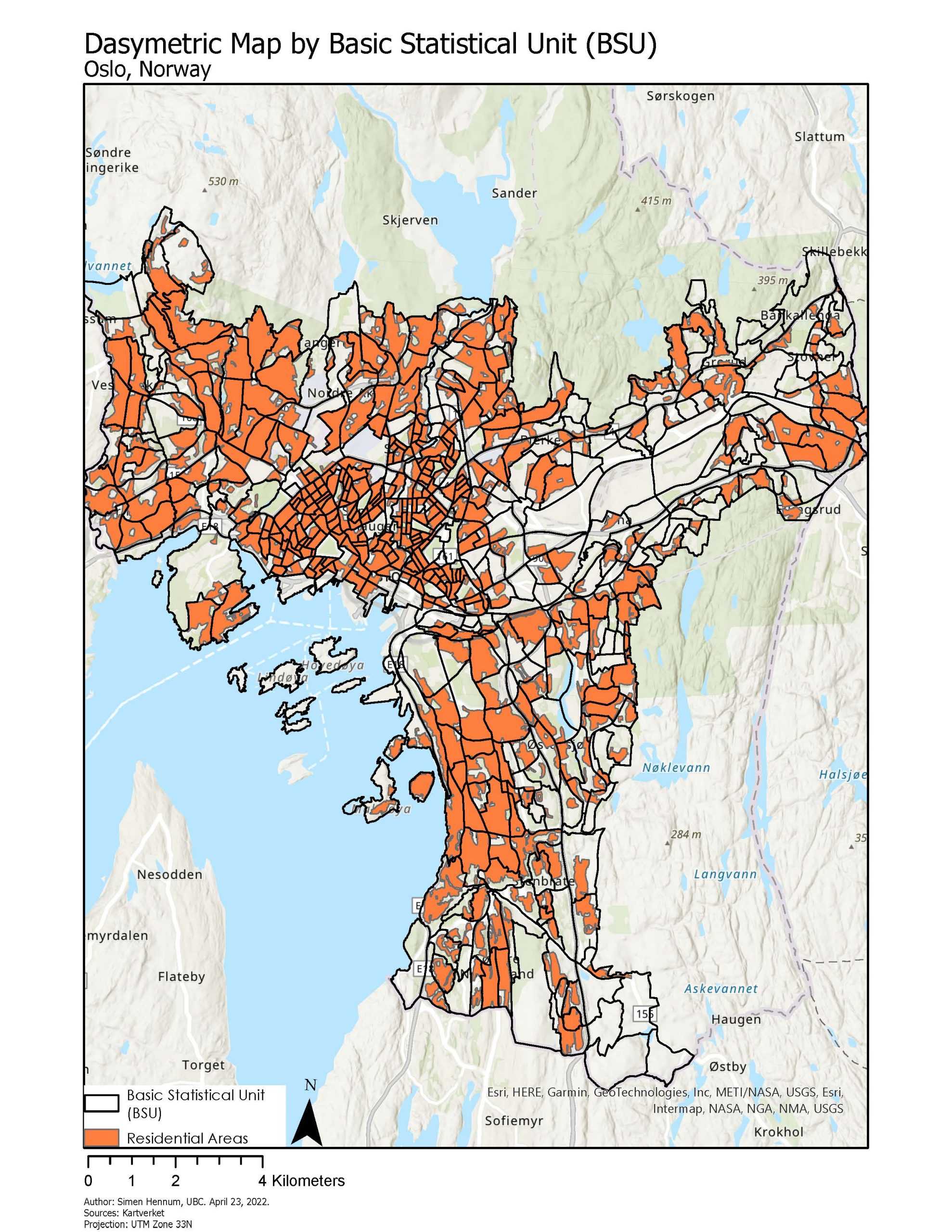
BSUs cover the entire extent of Oslo Municipality, including areas that are themselves sources of noise (e.g., industrial areas) and noise barriers (e.g., forests). In order to approximate the noise levels where people actually reside, I obtained land use maps from the Norwegian Mapping Authority and used the pairwise intersect tool to generate a dasymetric map of Oslo by BSU (Map 2). I assume that people are randomly distributed within the inhabited areas of each BSU. Given that the BSUs in most cases correspond to smaller city blocks in high density areas or larger, single-family units in smaller residential areas, this is a justified assumption.
Thus, two variables for each BSU, precent area/inhabitants exposed to sound above 55db and 80db were obtained.
At this stage in the analysis, I was faced with the issue of some of the variables being only available at a coarse spatial resolution (city district), while the noise levels were computed for BSUs. I computed the weighted average (according to population size) to obtain average noise values for each city district. As there are only 15 city districts, I would have too few data points to perform a meaningful regression analysis.
Thus, I chose to assume that the variables available only at the city district level are consistent across its spatial boundaries, allowing each BSU to obtain data point for all of the variables. While this is tantamount to ecological fallacy, it appeared to be the only way of conducting an analysis with enough independent observations.
In order to assess what candidate explanatory variables could best explain variation in sleep problems among Oslo youth, I ran the exploratory regression tool in ArcGIS Pro, using all the potential variables I originally retrieved (Table 1). The results of the exploratory regression led me to identify a model with the highest R2 and lowest AICc values (Table 2). Two variables (households with persistent low income and crowded households) showed evidence for multicollinearity.
Table 2: Initial exploratory regression analysis
|
Adjusted R-Squared |
Akaike’s Information Criterion | Max Variance Inflation Factor | Variables |
| 0.81 | 1691.20 | 1.54 | – Proportion of people exposed to noise >55db
– Wellbeing at school – Pleased with neighborhood – Children of single parents |
I ran an ordinary least-squares regression model using the variables identified with the exploratory regression tool. Spatial autocorrelation was assessed by calculating Moran’s I on the residuals (Map 3, Fig 1), and the data appear to exhibit spatial autocorrelation, indicating that a spatial explanatory variable might be missing from the analysis.
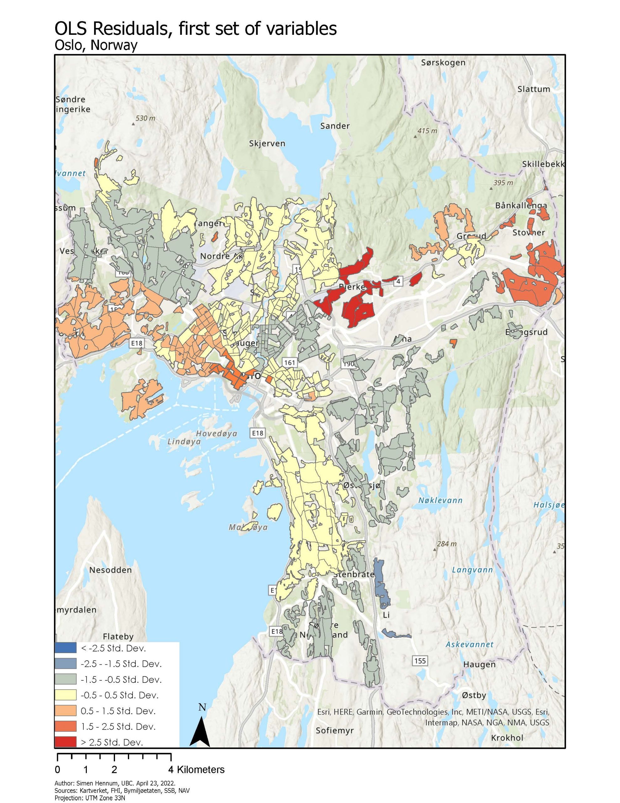
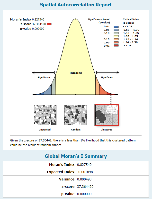 Fig 1. Spatial autocorrelation report of first OLS
Thus, I chose to include two additional spatial variables. The first, distance from major roadways with high speed limits (>70 km/h), railways, subways, and trams that are above ground (Map 4). While the noise map provided by Oslo municipality should account for these variables, it is possible that my translation of this data into a variable in the regression analysis is faulty.
![]()
I retrieved from Open Street Maps above-grounds roads with a speed limit higher than 70 km/h, railways, tramways, and subways. These were buffered with a distance of 75m in order to include in the subsequent step the BSU that are directly adjacent to but does not contain one of these features.
The second variable was distance to green spaces and forested areas, features that potentially reduce noise pollution levels. This was calculated using the land use map and the buffer tool.
I ran a second exploratory regression with the new spatial variables included. The model with the highest R2 and lowest AICc values included the new variables accounting for the distance from loud transportation features (Table 3). The variable accounting for proximity to green space was not included in this model.
Table 3: Final exploratory regression analysis
| Adjusted R-Squared | Akaike’s Information Criterion | Max Variance Inflation Factor | Variables |
| 0.81 | 1686.81 | 1.54 | – Proportion of people exposed to noise >55db
– Wellbeing at school – Pleased with neighborhood – Children of single parents – Within 75 meters of transportation feature |
Subsequently, I ran a generalized linear regression (GLR), assessed the spatial autocorrelation of the residuals of the GLR, and ran a geographically weighted regression (GWR). The results of these and their limitations will be discussed in subsequent sections.
Due to the limited utility of the results from these analyses, I performed a simple generalized regression at a finer spatial resolution, at the sub-district level, where income data is available. The results of this analysis will also be discussed in the subsequent sections of this report.
Next: results