Histograms for the variables included considered as candidate explanatory variables and the dependent variable were created in ArcGIS Pro (Fig 2). Most of the data is relatively normally distributed, except for the proportion of people exposed to decibels higher than 80db, which is to be expected.

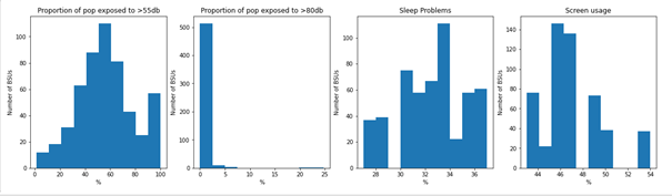
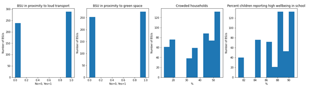
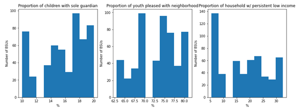
Fig 2. Histograms of variables

 

A table for pairwise correlations was computed (Fig 3). Of the candidate explanatory variables, BSUs with a high proportion of children with a sole guardian, crowded households, and households with persistently low income were the most strongly correlated with proportion of youth with difficulties sleeping (Fig 3). Other socioeconomic variables were also strongly correlated, indicating that Oslo is a divided city when it comes to living conditions and socioeconomics. Some of these variables exhibit multicollinearity

Importantly, the proportion of people exposed to noise levels above 55 and 80 decibels were not strongly correlated with any of the other variables. Weak correlations are apparent between neighborhoods with noise levels above 55db and neighborhoods with a high proportion of crowded households.

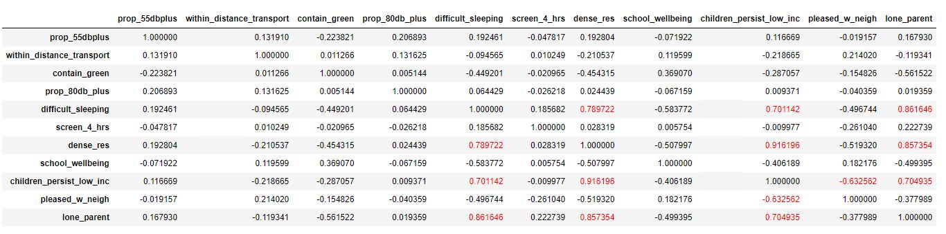Fig 3. Pairwise correlations with >0.6 highlighted in red

 

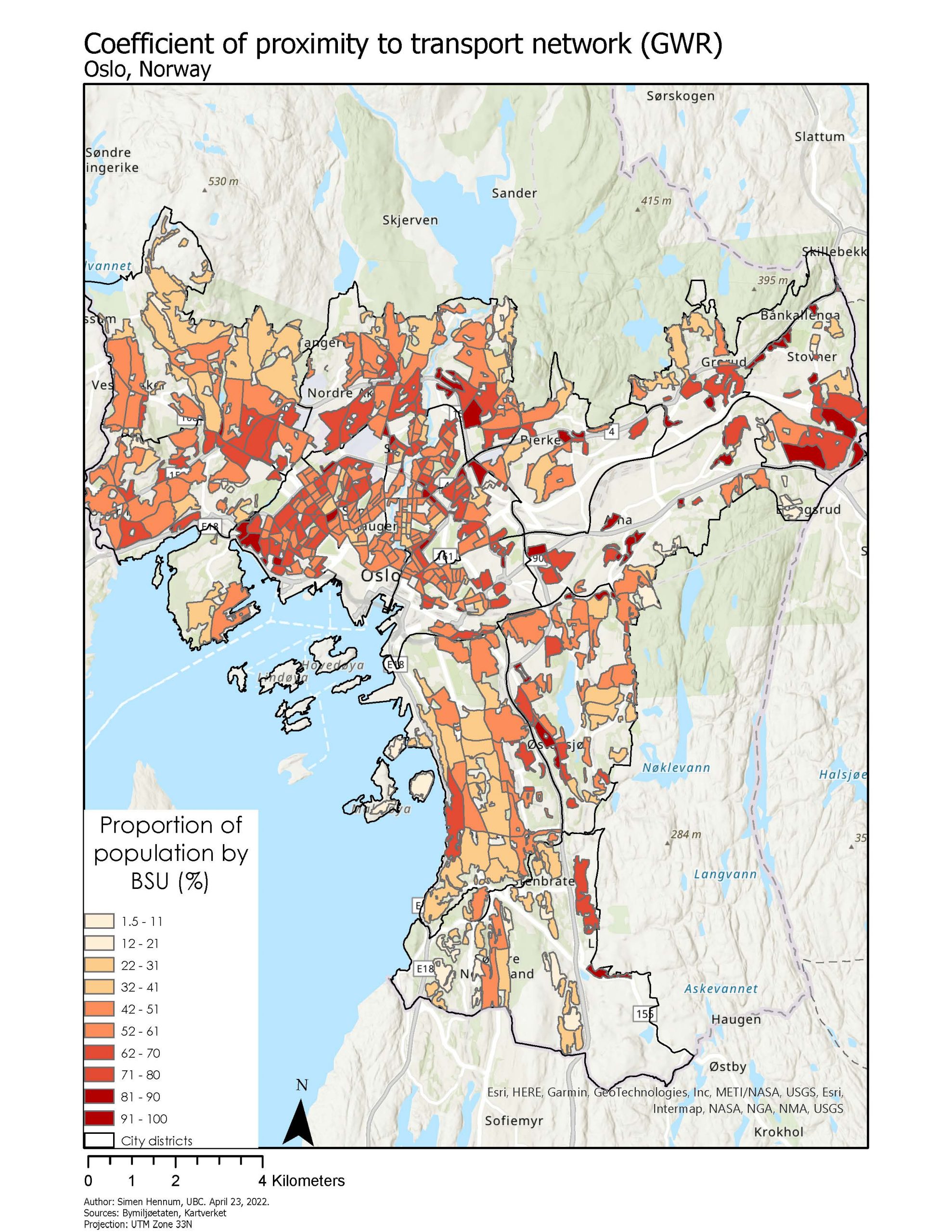
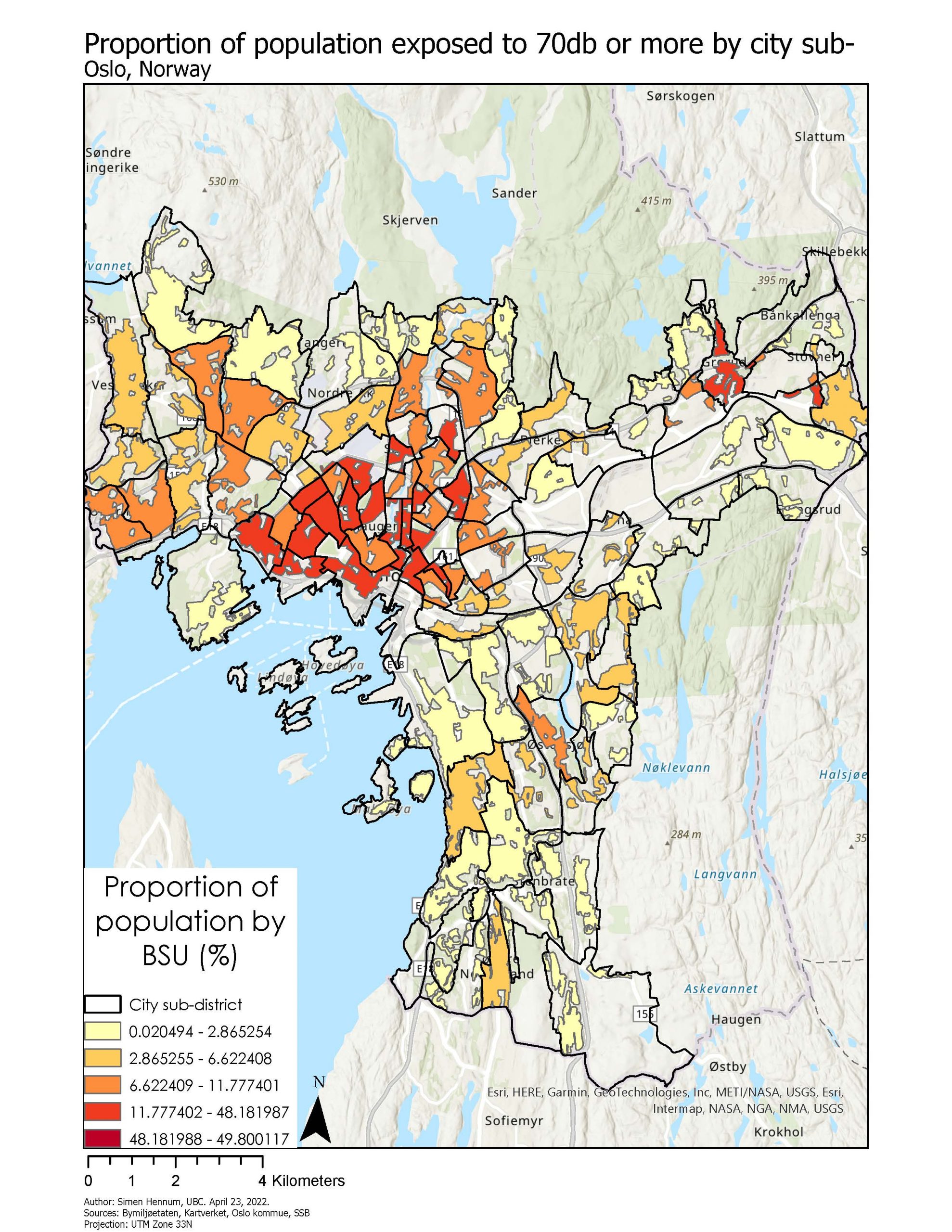
Noise pollution is most common around major roadways to the west, south, and north in the city (Map 1). The areas with high noise pollution are not necessarily the same areas as where people live. When calculating the proportion of an area covered by high noise levels, we can obtain maps with much greater detail of where people are potentially impacted by high noise levels (Map 5). Areas close to the city center, as well as to the west and east of the city, see a high proportion of area with high noise pollution.

Map 5 (full size)

 

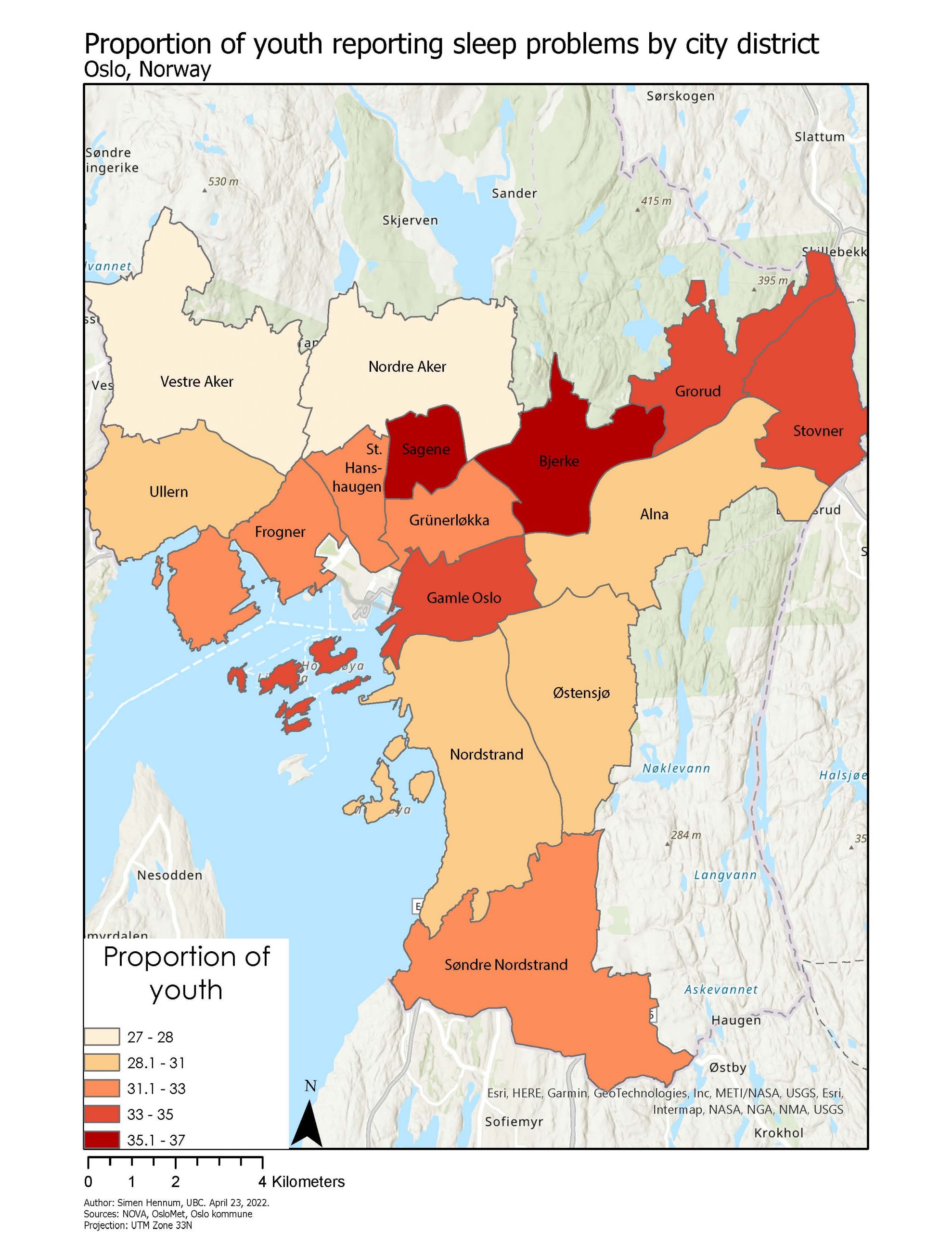
Sleep problems also appear to exhibit a spatial pattern where the city districts of Sagene and Bjerke have up to 37 % of youth reporting difficulties sleeping (Map 6), and city districts to the northwest of the city such as Vestre and Nordre Aker reporting proportions between 27-28 %.

Map 6 (full size)

Regression analysis

 

The results of the Generalized Linear Regression using the variables identified in the exploratory regression step indicate that the model is significant (Table 4, Table 5). The variables are all statistically significant, exhibit no multicollinearity, and report an R² value of 0.81. Wellbeing at school explains 21 % of the variation in sleep scores, indicating that in neighborhoods where youth are dissatisfied with school, sleep problems are more common. The same applies to being pleased with one’s neighborhood, with a coefficient of -0.11. Neighborhoods with higher proportions of children with a single guardian provides the most explanatory power for the variation of sleep problems in BSUs, with a coefficient of 0.59. Proportion of people living in a neighborhood with 55 decibels or more does not provide significant explanatory power, but is a significant variable. Neighborhoods with proximity to major transportation networks adds significant explanatory power to the model with a coefficient of 0.27.

Table 4: GLR coefficient summary

Variable	Coefficienta	StdError	t-Statistic	Probabilityb	Robust_SE	Robust_t	Robust_Prb	VIFc
Intercept	49.107828	2.259556	21.733394	0.000000*	1.783435	27.535534	0.000000*	——–
Proximity to major transport network	0.272638	0.107732	2.530700	0.011667*	0.105934	2.573656	0.010330*	1.079215
Proportion of population exposed t0 >55db	0.006608	0.002382	2.774734	0.005723*	0.002892	2.285236	0.022684*	1.054896
Wellbeing at school	-0.210991	0.021807	-9.675363	0.000000*	0.014766	-14.289274	0.000000*	1.339407
Pleased with neighborhood	-0.111704	0.010834	-10.310148	0.000000*	0.012297	-9.083639	0.000000*	1.208539
Lone Parent	0.590139	0.020565	28.696259	0.000000*	0.016335	36.126842	0.000000*	1.543503

 

Table 5: GLR diagnostic

Input Features	BSU Map	Dependent Variable	Sleep problem
Number of Observations	528	Akaike’s Information Criterion (AICc)d	1686.813443
Multiple R-Squaredd	0.814376	Adjusted R-Squaredd	0.812598
Joint F-Statistice	458.026847	Prob(>F), (5,522) degrees of freedom	0.000000*
Joint Wald Statistice	7819.141369	Prob(>chi-squared), (5) degrees of freedom	0.000000*
Koenker (BP) Statisticf	108.833112	Prob(>chi-squared), (5) degrees of freedom	0.000000*
Jarque-Bera Statisticg	117.217406	Prob(>chi-squared), (2) degrees of freedom	0.000000*

The Moran’s I for the residuals of the GLR are clustered, with a statistically significant Moran’s I at 0.77 (Fig 4). When running the spatial autocorrelation tool in ArcGIS Pro, I deemed that the conceptualization of spatial relationship that best works with this data is zone of indifference, where polygons not only in the same city district are considered in the calculation of Moran’s I.

 

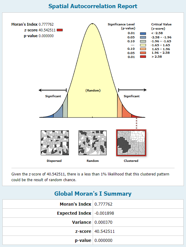
Fig. 4: Spatial autocorrelation report

The spatial clustering of the residuals may be due to the BSUs inheriting the values for some of the variables from their parent city district. That is, polygons have neighbors with identical data values for a few of the variables. When running the spatial autocorrelation tool at the city district level, the Moran’s I was not statistically significant, likely due to the few numbers of observations (n=15).

Interestingly, the model underpredicts sleep problems in areas surrounded by large transport networks, suggesting that the model is still not accounting for some of the spatial variables driving sleep problems in the city (Map 7).

Map 7 (full size)

 

Geographically weighted regression

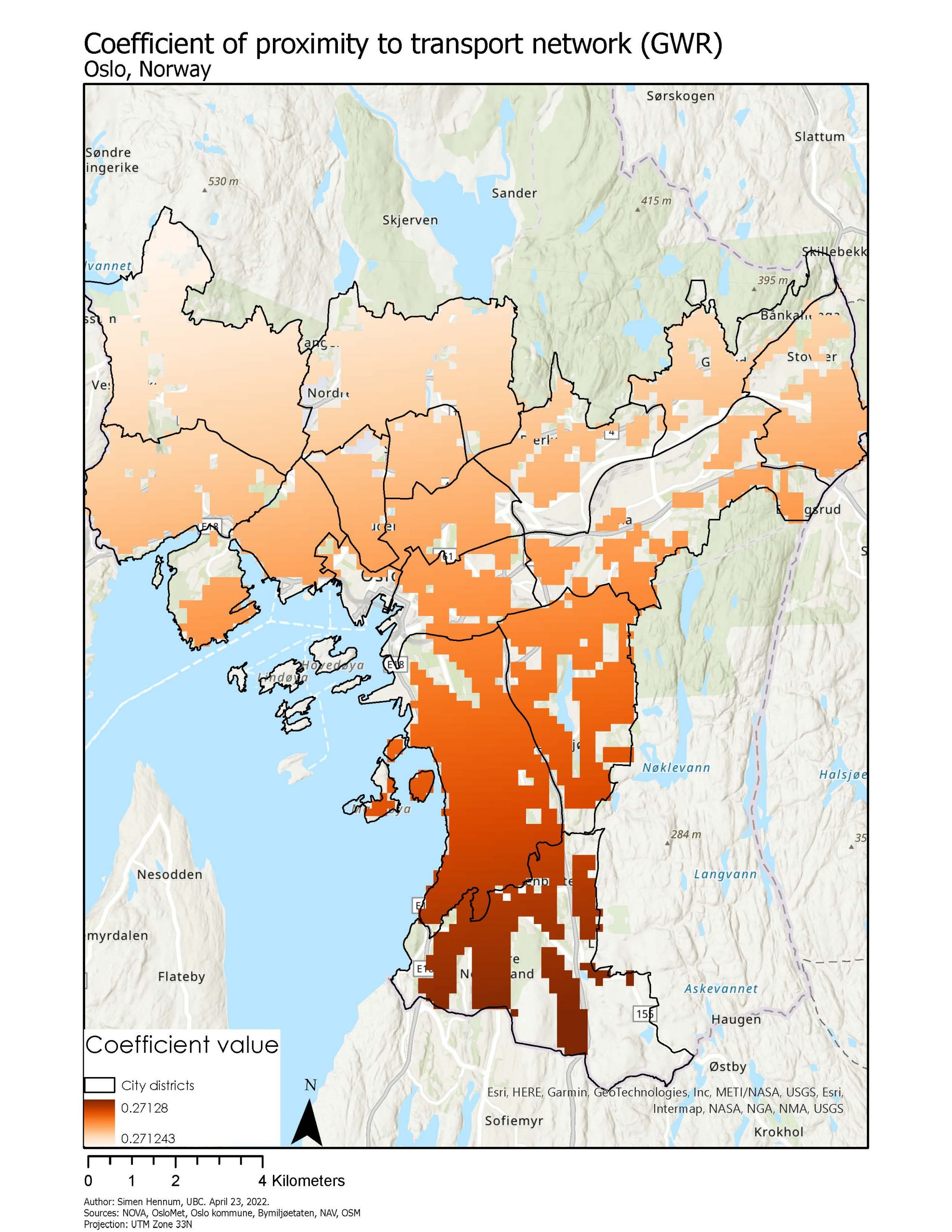
The results of the GWR do not provide particularly meaningful additional insight into the processes being studied. The variation of sleep variables was too low between different neighborhoods for the golden search method to detect at least one neighborhood. Only when defining the neighborhood type by a distance band of 100 kilometers, did the tool successfully run. The variation of coefficients between each area of the city was negligible (between 0.27128 and 0.271243 for proximity to transportation network) (Map 8, included for reference only).

Map 8 (full size)

 

Given that the GWR did not produce any meaningful results, I chose to explore whether there were any associations between noise levels and the one socioeconomic variable publicly available at a finer spatial scale – income. Using the same method as for the BSUs, I calculated the proportion of an inhabited areas of city sub-districts coinciding with noise levels above 55 and 70 decibels (Map 9). Income level was represented by the proportion of households with at least one child younger than 18 years old with low income (as defined by the European Union).

Map 9 (full size)

For both noise levels above 55 and 70 decibels, the weak positive associations between income and noise were not statistically significant (p-values of 0.76 and 0.43, respectively) (Fig. 5).

 

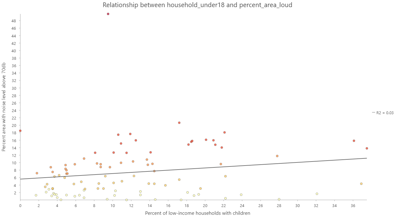Fig. 5: Scatterplot of income and noise level variables at city sub-district scale

 

Next: discussion & limitations