GIS plays an important role in crime mapping and law enforcement. This study looks at the spatial distribution of various crimes occurred in Nepean, Ottawa between January 2005 and March 2006 using a crime analysis program called CrimeStat. The effects of baseline population adjustment on the interpretation of spatial correlation were also explored in this study. The crime data was sourced from the Ottawa Police Department, whereas the dissemination area point data were derived from Statistics Canada.

Nearest Neighbour Analysis

The nearest neighbour index was first used to measure the spatial distribution of different crime types. This method generates the nearest neighbour index based on the average distance from each feature to its nearest neighbouring feature (Levine, 2013). Indexes that are less than 1 exhibit clustering, whereas indexes larger than 1 exhibits dispersion. In other words, the lower the nearest neighbour index, the more spatially aggregated the data is.

The distances between each crime (commercial break and entry, residential break and entry, auto theft) and their 25 closest instances of the same type of crime were analyzed. As shown in Graph 1, all of the indexes are below 1, meaning that the distance to the nearest crime of the same type is less than what would be expected in random conditions, thus all the data are spatially aggregated. Furthermore, these three crimes display a decreased correlation as the chose point is farther away. The closer the neighbouring cell, the more spatially aggregated crime occurrences are. This pattern is most apparent within the first five orders. Commercial break and enter appears to be more concentrated (0.19) than car theft (0.26) and residential break and enter (0.29). This could be explained by the land uses the arrangement in Nepean, Ottawa. Commercial land uses are more concentrated, especially around the downtown area . Stores and shopping centers that are prone to break-in are usually located in close proximity to each other in commercial areas. As a result, commercial break and enter follow a similar spatially aggregated pattern. Downtown population centers are also where cars generally cluster, resulting in the aggregation of car thefts spatially. On the other hand, residential crimes have a slightly higher index—meaning a more dispersed distribution—as residential areas span over a larger area and are more dispersed. This segregation can be caused by a range of factors, such as property values and accessibility.

Graph 1. Nearest Neighbour Index for residential break and enter, commercial break and enter, and car thefts.

 

Moran’s I

While nearest neighbour analysis looks at the presence of clustering in crimes data by the individual data points themselves, Moran’s I allows us to examine the distribution of crimes in relation to an area, in this case, the dissemination areas of Ottawa. Under Moran’s I analysis, crimes are aggregated to the geographic unit of a dissemination area (Levine, 2013). The tool computes the mean and variance for the attribute being evaluated, compared that to the value of the variable at any one location with the value at all other locations to see how one object is similar to others surrounding it (Levine, 2013). Moran’s I can range from -1 (perfect dispersion), to 0 (complete random distribution), to 1 (perfect spatial autocorrelation). In other words, the higher the Moran’s I, the more spatially aggregated the data is.

The Moran Correlogram below compares the intensity values (Moran’s I) of 4 variables: commercial break and entry, residential break and entry, auto theft, and population (total population above 15). It shows how concentrated, dispersed, or randomly distributed is the spatial autocorrelation of each crime types compared to the baseline population. 200 distance intervals were used. Across the 3 crimes, the data shows that the dissemination areas with high crime intensity are mostly surrounded by dissemination areas that also have high crime intensity, and the closer the dissemination areas, the more spatially autocorrelated they are. All of the I values drop until it reaches 20km. This echoes with the result generated by the nearest neighbour analysis. The I value at zero distance is the highest for residential break and enter (0.325), then car theft (0.07), followed by commercial break and enter (0.025). This means that the occurrence of residential break and enter is most correlated to their surrounding neighbours, at least for short distances. Interestingly, this result contradicts with what was concluded in the nearest neighbour analysis. One of the explanations to this inconsistency is that, although residential break and enter crimes do not correlate strongly with each other over a large area of dispersed land uses, they are similar at a smaller scale within each dissemination area of Ottawa.  It is also worthy to note that the three crimes’ intensity values are higher than that of the population (which is the null value). This means that these crimes are more clustered than what would be expected, and the clustering is not merely a function of population density.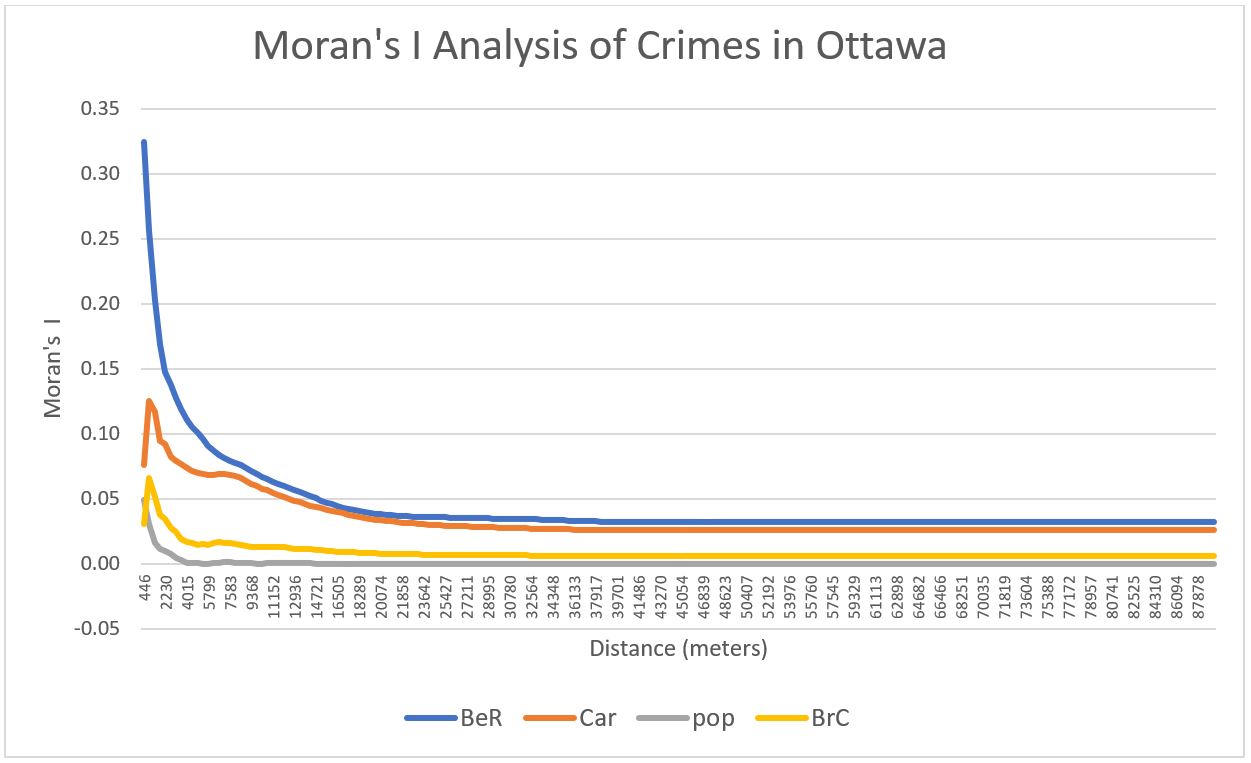

Graph 2. Moran’s I of residential break and enter, commercial break and enter, and car thefts.

 

Hot Spot Analysis

Fuzzy mode and Nearest neighbour hierarchical spatial clustering

The occurrence and frequency of crimes were then examined using two hot spot analysis methods: fuzzy mode cluster and nearest neighbour hierarchical spatial clustering. Fuzzy mode cluster uses point locations as the basis for clustering. Locations with the greatest number of incidents are defined as hot spots (Levine, 2013). Fuzzy mode allows users to define a small search radius around each location to include events that occur around or near that location but without precise measurement; hence, it is known as a ‘fuzzy’ approach (Levine, 2013). While Fuzzy mode represents crime frequencies as point data, nearest neighbour hierarchical spatial clustering represents frequencies in hot spot polygons. Nearest neighbour hierarchical spatial clustering statistically delimits hot spots using a hierarchical technique. The hierarchical technique functions like an inverted tree diagram in which two or more incidents with the highest level of similarity (spatially) are grouped together (first order), then these first order clusters are further grouped into larger second-order cluster, until all incidents converge into a single cluster.

Figure 1 shows the hot spots calculated using both the fuzzy mode (points) and nearest neighbour hierarchical spatial clustering (ellipse). For the fuzzy mode, crimes within 1000 meters around a location were investigated. The results were coloured according to the density of crimes, ranging from 1-32 other crimes located within 1000 meters (green dots), to 61-100 other crimes located within 1000 meters (red dots). These points allow us to visually observe the presence of spatial autocorrelation and identify hotspots in locations where points, especially red points, cluster. Nearest neighbour hierarchical spatial clustering, on the other hand, gives a statistical account for crime hot spots. Areas within 1000m of a location with a minimum of 10 points are identified and bounded by blue ellipses (Figure 1). These ellipses show hotspot patterns that are not easily identified using the fuzzy mode. Elongated ellipses are mostly found along highways and main roads, indicating a linear distribution of crimes; while circle ellipses are found in urban centers in the downtown areas. Nevertheless, the locations of the ellipses closely resemble that of fuzzy point clusters.

 

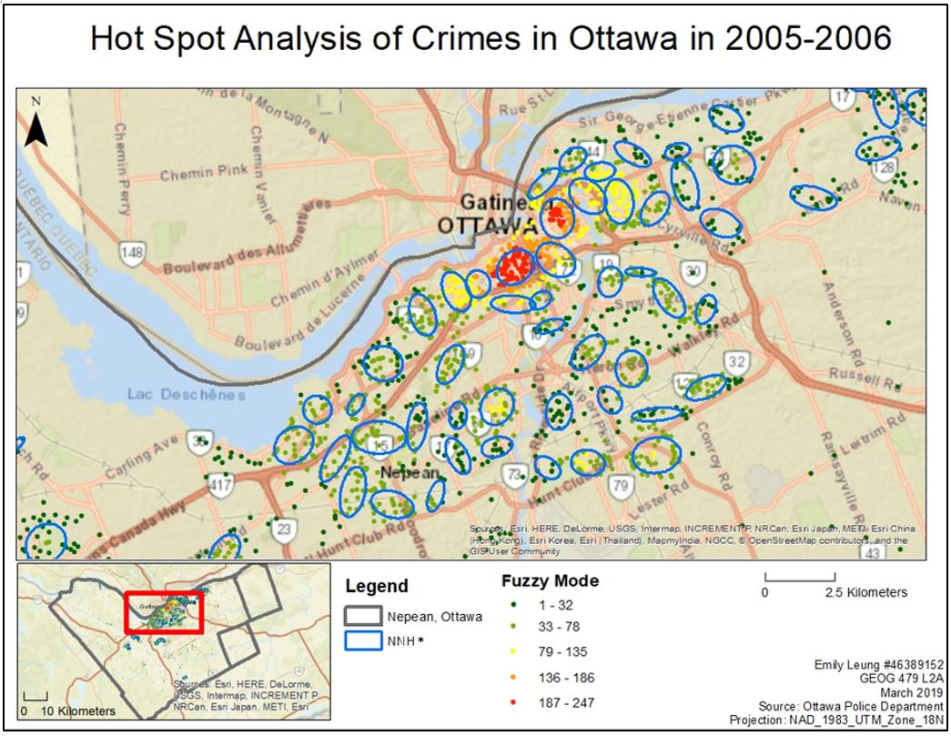
Figure 1. Hot spot analysis: a comparison between fuzzy mode and nearest neighbour hierarchical spatial clustering of Residential Break-in Crimes in Nepean, Ottawa

 

 

Standard and Risk-Adjusted Nearest Neighbour Hierarchical Spatial Clustering

Hot spot analysis using standard nearest neighbour hierarchical spatial clustering can be limited as it does not account for the underlying variables that may skew the total or non-normalized data. For example, a cluster of crimes could be a result of high population density or low median income around city centers. In situations where the volume of crimes fails to tell us the full story of crime occurrence, measurements of the relative risk of crimes become vital. For this reason, risk-adjusted nearest neighbour hierarchical clustering was used to fill the gap. This method allows clusters closer than what would normally be found in a certain baseline population to be identified (Kumar & Chandrasekar, 2010). In other words, the results are normalized based on the baseline variable, in this case, the population aged 15 years old and above in a dissemination area (assuming that most crimes were committed by this age group). Sparsely populated areas with high relative crime rates would be classified as hot spots under this method.

The risk-adjusted map identifies 3 orders of clusters (Figure. 2). First-order clusters are statistically clustered based on the same criteria used in standard nearest neighbour hierarchical spatial clustering. The second-order clusters, in turn, are clustered into third-order clusters. The re-clustering process reveals three levels of grouping: specific hot spot locations (first-order cluster), specific areas in the city (second-order cluster), and finally the central high-risk area located in downtown (third-order cluster). The breaking down of crime data into 3 different levels allows for both general and specific analysis of crime hot spots.

Figure 2. risk-adjusted nearest neighbour hierarchical spatial clustering of residential break-in crimes in Nepean, Ottawa

 

Kernel Density Interpolation

Departing from point-based (fuzzy mode) and polygon-based (nearest neighbour hierarchical spatial clustering) analyses, kernel density analysis offers new insight into the residential break and enter crimes dataset by producing a continuous surface of crime density in Nepean, Ottawa (Kloog et al., 2009). The surface was produced by interpolating the crime data over the entire area using triangular distribution. This tool evaluates the distance between reference cells and residential break and enter locations, calculates the kernel function for each measured distance, and then sums the values of all surfaces for that reference cell (Levine, 2013). It calculates the densities for all locations, hence, gives a more holistic view of the data and facilitate a more accurate way of identifying micro-level areas of risks.

Similar to nearest neighbour hierarchical spatial clustering analyses, Kernel density interpolation analysis was split into two parts: single and dual-kernel density routines. Single kernel density concerns about the absolute distribution and density of crimes locations, which is comparable to nearest neighbour hierarchical spatial clustering (Figure. 3). The red areas indicate a high density of crimes committed or hot spot clusters. A very high concentration residential break and enter incident is found within Ottawa West, Ottawa West Centretown and Ottawa Central. However, this concentration could simply be a reflection of the high population density in these downtown areas. More complex analysis is therefore needed. Like the risk-adjusted nearest neighbour hierarchical spatial clustering analysis, dual kernel density method recalibrates crime density based on a second variable, which is population above 15 years old (Figure. 4). It looks at the risk of crime, rather than the volume, given the underlying population for the entire area. Two surfaces—one for crime instances and another for population—were produced simultaneously (Zusman et al., 2016). Next, the kernel density estimates for residential break and enter was divided by the kernel density estimate for the population for each reference cell location (Zusman et al., 2016). While there is still a concentration of thefts in the center, it’s more spread out and a new cluster in Ottawa South is identified (Figure. 6). These two maps are complementary to each other in identifying areas with a high total number as well as high risk of crimes (based on their population size).

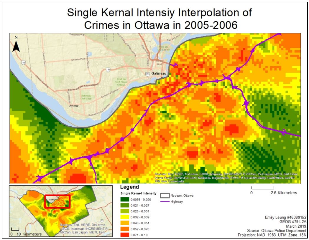
Figure 3. Single Kernel Density of Residential Break-in Crimes in Nepean, Ottawa

Figure 4. Dual Kernel Density of Residential Break-in Crimes in Nepean, Ottawa

Spatial and Temporal Clustering

Knox Index

For the car theft data, Knox index was used to examine both the temporal and spatial relationships between incidents. This tool compares two points at a time and divides them into groups based on 2 criteria: (1) distance—whether car thefts are close or not close in space—and (2) time of day the crime was committed—whether thefts are close or not close in time (Levine, 2013). CrimeStat generates a Chi-Squared statistic that compared the expected model and the actual values of the data (Levine, 2013). The actual observed Chi-square value is 94.01612; whereas the maximum random Chi-squared value is 3.53003. The high Chi-squared value demonstrates a significant departure from the random model, and as the Chi-squared value is much higher than the expected, this pattern is statistically significant. This is further confirmed by the p-value. The p-value of this analysis is 0.00010, meaning that only 0.01% of the time does this model is resulted by chance (Levine, 2013).

The Knox analysis ran 19 times to examine car thefts which are within 6 hours and 5 km of each other. This analysis assigns each pair of points into one of four categories: close in time and space (325473); not close in time and space (759110); and close in time and not close in space (986929); and not close in time and close in space (242964).  The analysis shows that car thefts are most likely to be not close in space, but close in time. This means that the policing effort is most effective when focused at times when crimes happen frequently rather than a specific location where cars are mostly stolen.

 

References

Levine, N. (2013). CrimeStat IV: A Spatial Statistics Program for the Analysis of Crime Incident Locations (version 4.0). Ned Levine & Associates, Houston, TX, and the National Institute of Justice, Washington, DC.