2.1 Data Acquisition

It is important to stress that we are working in a fictional universe. Fortunately, there exists a dedicated Lord of The Rings fanbase (which includes cartographers!) that has created many GIS interpretations of Middle Earth. The Middle Earth DEM Project (https://forum.outerra.com/index.php?topic=1491.0) was created by a group of individuals who set out to create a high resolution DEM of Middle earth.

Unfortunately the Middle Earth DEM project was taken off the web in 2014. Through some searching, we were able to find the shapefiles (common place names, hydrology, forests, roads) from the project on GitHub, which were properly georeferenced. All of this data, being imaginary, was hand-drawn and of only mediocre quality. Rivers did not connect or terminate properly, and what should have been closed polygons were actually many small lines. However, these data formed the backbone of our DEM georeferencing.

After a bit more searching, we found a 8-bit heightmap with values of 0 – 255 in black and white, which represented elevation. Each heightmap value represents roughly 19 metres of elevation. That is to say, a value of 1 in a cell (black) is equal to approximately 19 m, and a value of 255 (white) is equal to approximately 4,800 m. These are not elevations above sea level, but elevations above seafloor. This allowed us to create our own DEM off the .jpg image, and georeference it appropriately (Figure 2.1). Mount Doom was used as the normalizing elevation factor, as it is a known elevation (1371.6 meters above sea level).

Figure 2.1 Greyscale elevation basemap of Middle Earth used to create DEM. Resolution across entire image = 2000km.  (Source: http://worlds.outercraft.com/forum/index.php/topic,27.60.htm.)

Interestingly, despite working in a fictional world, we were able to georeference our height map DEM to the real world. J.R.R. Tolkien stated that the mill at Hobbiton is inspired by Sarehole Mill in Birmingham, England, where he lived for a period in his childhood. The guideline we used (http://gisninja.blogspot.ca/2012/12/georeferening-middle-earth.html) also georeferenced Minas Tirith to Florence, Italy (Figure 2.2). With this information, we could confidently georeference the heightmap to the shapefiles. By selecting 6 points across the heightmap, corresponding to the corners of lakes (easily identifiable on both layers), we could match the two points on each layer to determine the surface transformations required to properly display them.

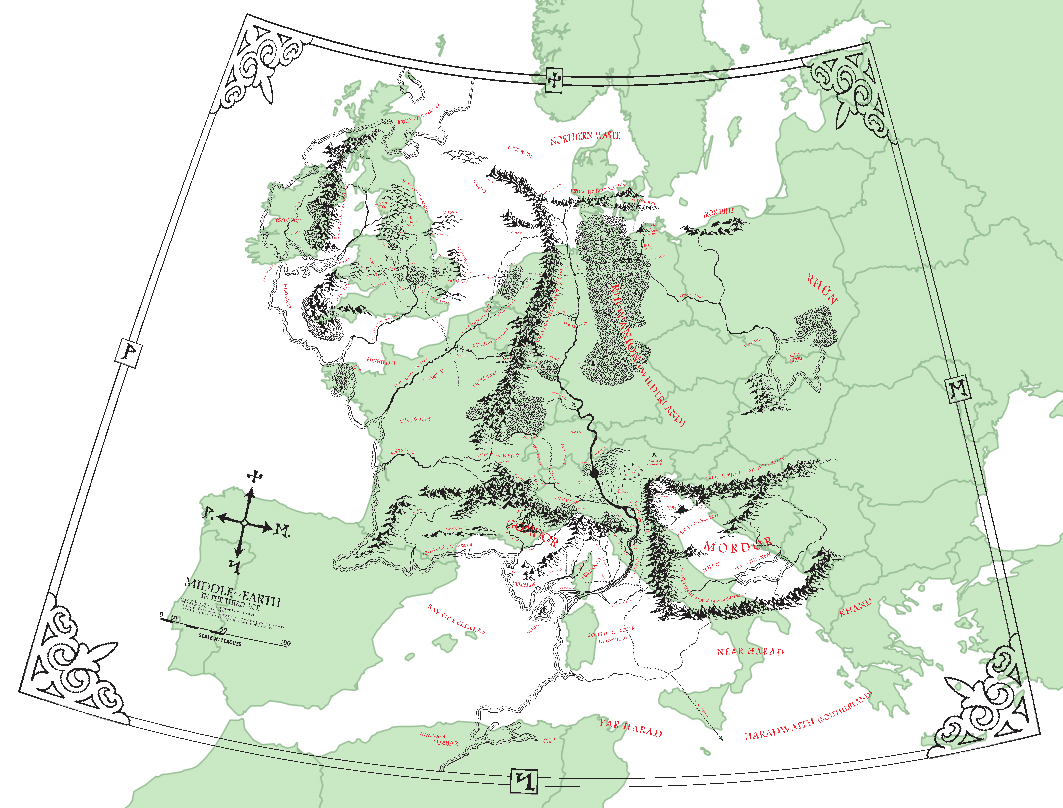
Figure 2.2 Middle Earth georeferenced to Europe (Source: http://gisninja.blogspot.ca/2012/12/georeferening-middle-earth.html).

2.2 Creating a Model

Armed with our DEM and feature data, we began to build our model. The model itself had one major goal: it must accurately represent the social and physical factors affecting the hobbits’ path, while obeying our time and resource constraints.

To make sure that we are comparing like values, we normalized all of the factors to some multiplier of the hobbits’ walking speed. For example, walking through the forest without a path slows them down, and so the forest’s speed modifier is 0.5, or 50% of their base walking speed. This allows us to attempt to quantify the relative strength or importance of the various factors.

2.3 Determining Speed Modifiers

Our speed modifiers were broken down into two classes: Physical (P) and Social (S). The assigned speed modifiers are listed below:

Factor	Class	Speed modifier (0% – 100% of the hobbits’ walking speed), values above 100% can be obtained by taking a boat along a river (downstream).
Forest	P	Assuming trackless, 50%
Rivers	P	Crossing: 50%; Travelling down: 200%
Hills	P	(wrapped into the slope surface)
Roads	P	P =100% (Includes bridges
Mountains	P	(wrapped into the slope surface)
Snow	P	25% (depends on thickness of snow, assuming roughly 0.5 m of snow depressed until it is compact enough for a hobbit to walk on).
Moor	P	75%
Lake/Ocean	P	10%
Hostile Region	S	60%, actually bad idea because of Easterling traffic travelling down from Rhun
Roads	S	80% (Moving cautiously, they don’t actually need to be off the road until a nazgul is close to them)
Nazgul	S	10% (20 km buffer)
Hostile Town	S	Buffer zone with tiers of 10 / 25 / 50 km (25% / 50% / 75% respectively)
Hostile Army	S	Buffer zones with 5 / 10 / 15 km (25% / 50% / 75% respectively)
Danger Zone	S	90% (Accounts for random encounters with monsters, bandits, minor environmental hazards, etc. Allows for faster travel and preferred routing towards friendly territory)
Friendly Town	S	Buffer zones of 10 / 25 / 50 km (100% / 95% / 92.5% respectively)
Friendly Army	S	Buffer zones of 5 / 10 / 15 km (100% / 95% / 92.5% respectively)
Friendly Creature	S	Buffer zones of 2 / 4 / 6 km (96% / 94% / 92% respectively)
Hostile Creature	S	Buffer zones of 2 / 4 / 6 km (84% / 86% / 88% respectively)
Friendly Region	S	95%

2.4 Sensitivity Analysis and Weighting of Factor Classes

In the creation of our least cost paths, we chose to include 18 types of factors that would influence the route taken. After classifying the factors into 2 classes (physical and social), sensitivity tests were conducted to determine which weight we should give each class in the final friction surface. We experimented with three different weighting schemes:

1. Equal (50% Social, 50% Physical)
2. Social (70% Social, 30% Physical)
3. Physical (30% Social, 70% Physical)

Equally weighted physical and social factors were determined to be the best weighing strategy, after an analysis of cost paths with different weights (Figure 2.3). The slope calculation is expanded upon further in section 2.6.

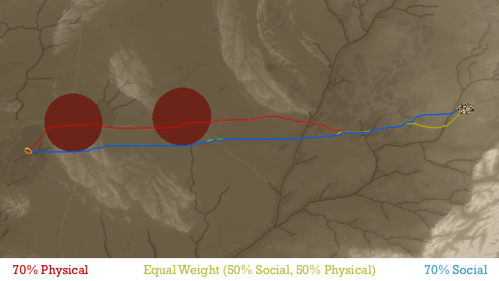
Figure 2.3 Class Weight Comparison

This initial comparison was key in determining our final weighting. The large red circles are the locations of Nazgul during the first week of our analysis. Although the red line (Physical-preferred) most closely approximates the actual path of the story, both the green (Equal weights) and blue (Social-preferred) are much safer. We ultimately chose an equal-weighted scheme because of illogical behaviour of the socially-weighted path.

For example, the social path ignores the road even when there is no danger on it. However, the equal path will take the road, provided there is a physical benefit. This can most clearly be seen as the two paths approach Rivendell. When there is significant danger, the equal path will follow the socially optimal route. When the danger subsides, however, it switches over to following the physically optimal route. This was our desired behaviour, and so our final map uses an equal weighting of both social and physical factor classes.

2.5 Generating Factor Classes

The factors themselves were generated as a series of rasters, with values equal to their speed modifiers where relevant, and zero everywhere else. For our point sources (Towns, armies, etc.), multiple ring buffers were used to simulate spheres of decreasing influence and/or troop density. For example, the closer we get to Isengard the higher the danger, and so the higher the friction (and lower the speed).

From there, we use Cell Statistics to calculate the mean speed modifier for each friction class. See figure 2.4 for an example of a social friction layer. White represents low friction, and black represents high friction. Note the grey background covering the majority of the map, this represents the danger of the wilderness. We assume some randomness in events that befall the group, including things like bandits, storms, broken wheels, etc. We estimate that these events will, on average, reduce their travel speed by roughly 10% while in the wilderness. As they approach civilization, however, roads improve, guard patrols reduce the presence of bandits, friendly inns and establishments make life easier in many ways, and so we expect their speed to, on average, increase close to friendly towns relative to the wilderness.

There is one exception to the Cell Statistics (Mean) part of this calculation. The Nazgul layers are prioritized above all else, and so we use Cell Statistics (Minimum) to take the minimum of the social friction layer and the Nazgul layers.This yields the intense dark spots in figure 2.4, below.

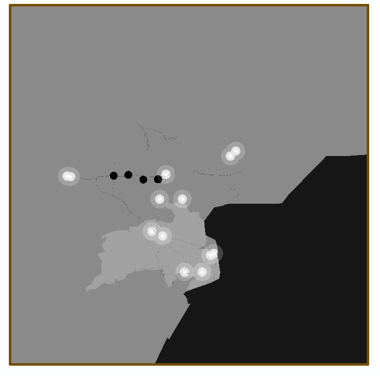
Figure 2.4 Social Friction for Step One

Once the friction surface is built for both friction classes, they are then averaged together, through Cell Statistics (Mean). This gives us our final friction surface. However, these values are speed modifiers, represented as the average speed reduction (in percent) experienced when traveling through each cell. To convert this to a cost for the least-cost path analysis, we perform a simple mathematical operation:

Friction Cost = 200 – (Speed Modifier * 100)

This gives us a friction value that is high if the speed modifier is low, and low if the speed modifier is high. It is a linear function, with a theoretical minimum value of 50 [Friendly Army (S) + Boatable Area (P)], and a theoretical maximum value at 190 [Nazgul (S) + Lake (P)].

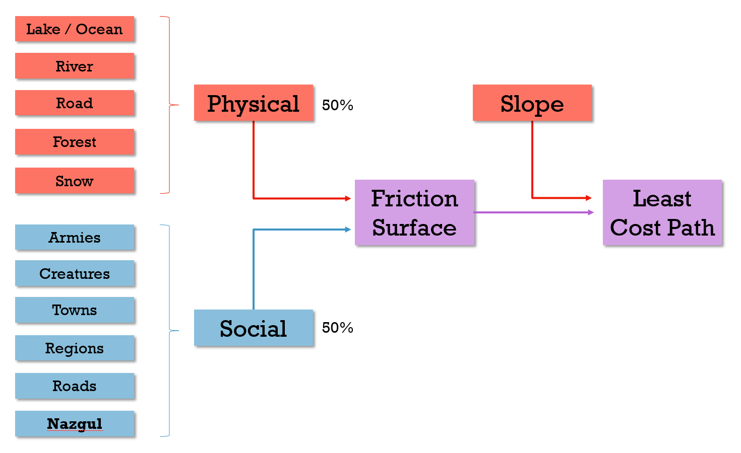Figure 2.5 Generalized Procedure Flowchart

2.6 Creating an Anisotropic Surface

To make our analysis realistic, we include slope as a factor in influencing travel speed, as it is much slower to travel uphill than it is to travel downhill. Because the Misty Mountains are an important topographic feature in Middle Earth, and would need to be crossed to get to Mordor from Rivendell, this becomes an especially critical factor in Frodo’s route.

A simple slope map would not suffice for our analysis, however. The slope of a hill depends on which direction you are moving across the hill. For example, moving uphill is significantly harder than moving across the hill. Because of this directional dependence, we had to use the vertical factor function built into ArcMap. Firstly, a slope function had to be determined. We used the symmetric inverse linear slope function as our vertical factor (Figure 2.6). This calculates the value for the slope in the direction of motion, and multiplies the friction value of the cell by the Vertical Factor. Thus from Figure 2.6 it is clear that a higher slope means a higher friction cost.

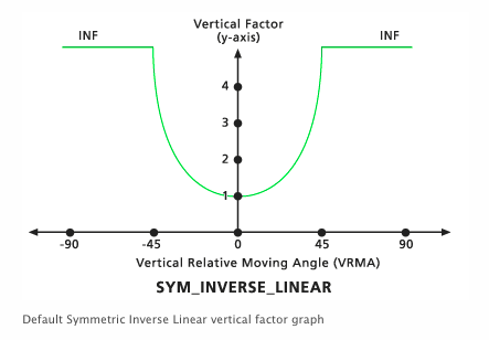
Figure 2.6 How the horizontal and vertical factors affect path distance, ArcGIS Help. (Retrieved from: http://desktop.arcgis.com/en/arcmap/10.3/tools/spatial-analyst-toolbox/how-the-horizonal-and-vertical-factors-affect-path-distance.htm)

Unfortunately, because the slope factor cannot be accounted for in our friction surface (and so in our weighting of social and physical factors, see Figure 2.5), we had to change the effect of the vertical factor based on the weight that we were using. We chose to modify the slope of the symmetric inverse linear function, as well as the high and low-cutting angle, or the maximum allowable slope. This has the effect of reducing the range of the Vertical Factor when the social class is more heavily weighted, and increasing it proportionally when the physical class is more heavily weighted.

The default slope is -1/45, the default low-cutting angle is -45, and the default high-cutting angle is 45.  We changed these values to reflect the different weights, as seen in Figure 2.7.

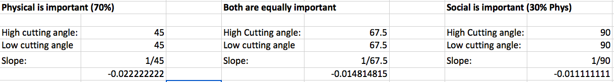
Figure 2.7 Three Weight Schemes and Their Respective Angles and Slopes.

2.7 Moving Along the Path

Once we have created our friction surfaces, calculated the vertical factors, and run our path distance, we reach the point where we must move along the path by two weeks of time.

To do this, we average the friction costs across the path and convert that to an average speed. This is the same as the equation outlined in step 2.5, but in reverse. An example calculation is outlined below.

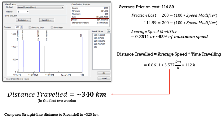
Figure 2.8 Example Calculation for Distance Traveled

Once we have an average speed, we can then calculate the approximate distance moved along the path, assuming a day of travel is about eight hours spent walking at the average speed. Once we have moved the hobbits 14 days along their path, we repeat the whole process over again for the next time step, moving armies and creatures as necessary and recalculating the friction surfaces.

2.8 A Shifting Sociopolitical Landscape

As you can see in figure 9 below, there are many social features dotted over the landscape. As we move the hobbits through time, so too must we move the notable or relevant barriers. For each time step, we represent the creatures at all points at which they appear for a given period. For example, between the 24th of September 3018 and the 11th of October 3018, Nazgul appear four times in the book. Thus, for that time period, we have four Nazguls represented on a single friction map.

This is the largest consequence of our “limited omniscience” approach to Frodo’s perception. He not only knows where the Nazgul are currently, but where they will be. This allows the path to avoid constant recalculations as the nazgul chase him, reducing the workload of running the model to a manageable amount.

We could, in theory, recalculate the friction surface for every time a Nazgul moves, but that would result in a much higher number of maps, and is somewhat beyond the scope of this particular project.

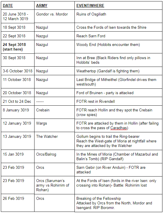
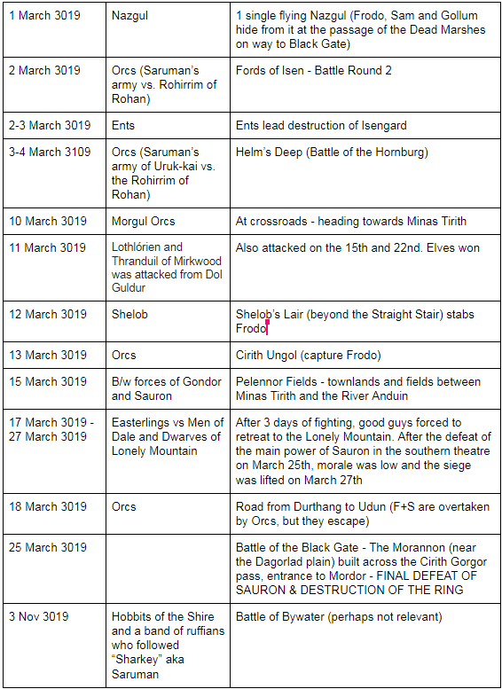
Figure 2.9 Timeline of the events of The Lord of the Rings trilogy. Referenced from http://lotrproject.com, as well as the books and movies.