Data Preparation:
Note: All data layers were projected to NAD 1983 UTM Zone 17N (Data Management > Projections and Transformations > Project).
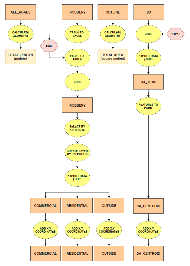
Figure 1. Flowchart showing data preparation process in ArcMap 10.6.1.
CrimeStat 4.02:
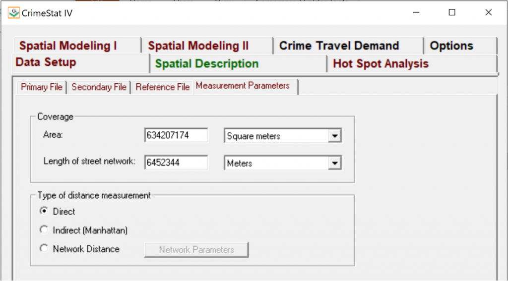
Using the geometry calculations from ArcMap 10.6.1 for City of Toronto land area (square meters) and length of street network (meters), the Measurement Parameters for CrimeStat were set to the following:
- Area (square meters) = 634 207 174
- Length of street network (meters) = 6 452 344
1) Nearest Neighbour Analysis: The nearest neighbour index (NNI) is a distance statistic that compares the nearest neighbour distance, i.e., the average distance between nearest points, and the mean random distance, i.e., the nearest neighbour distance expected on the basis of chance (Levine, 2013). If the observed average distance is the same as the mean random distance (i.e., evidence of spatial randomness), the NNI will equal to 1.0. If the observed average distance is smaller than the mean random distance (i.e., evidence of spatial clustering), the NNI will be less than 1.0. Conversely, if the observed average distance is greater than the mean random distance (i.e., evidence of dispersion), the NNI will be greater than 1.0.
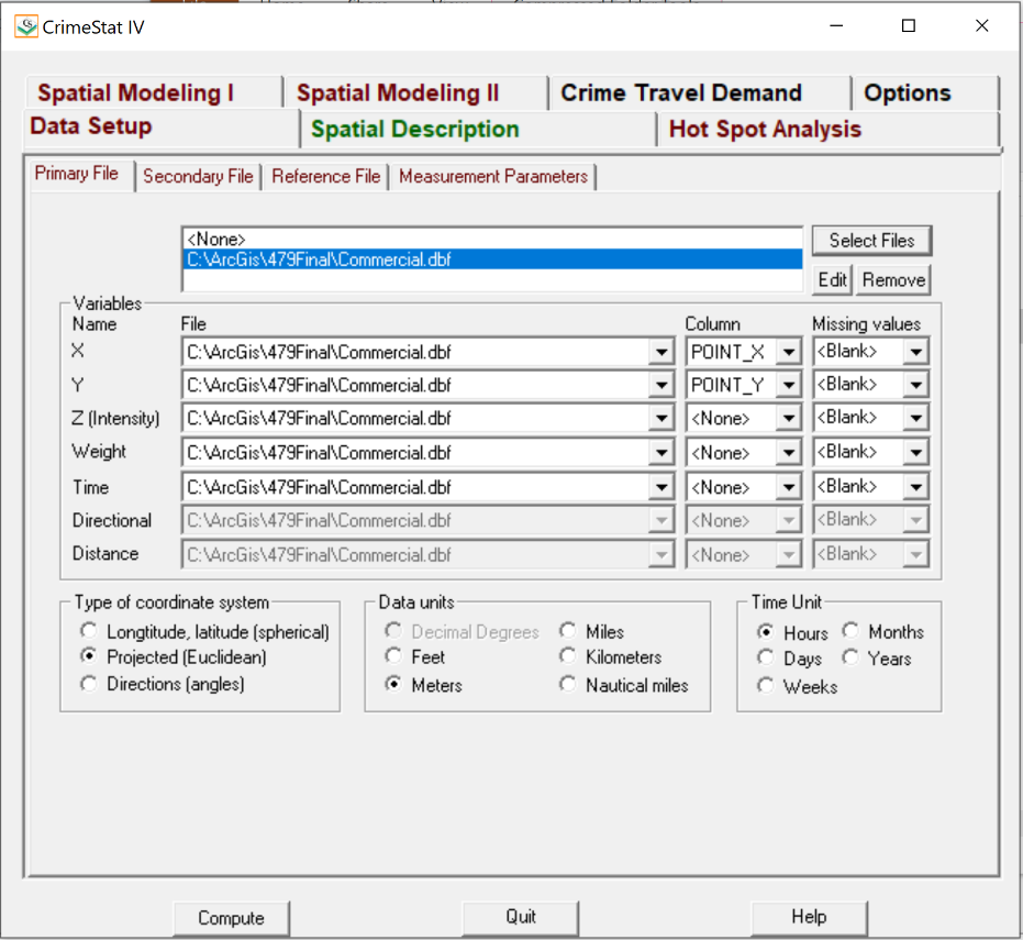
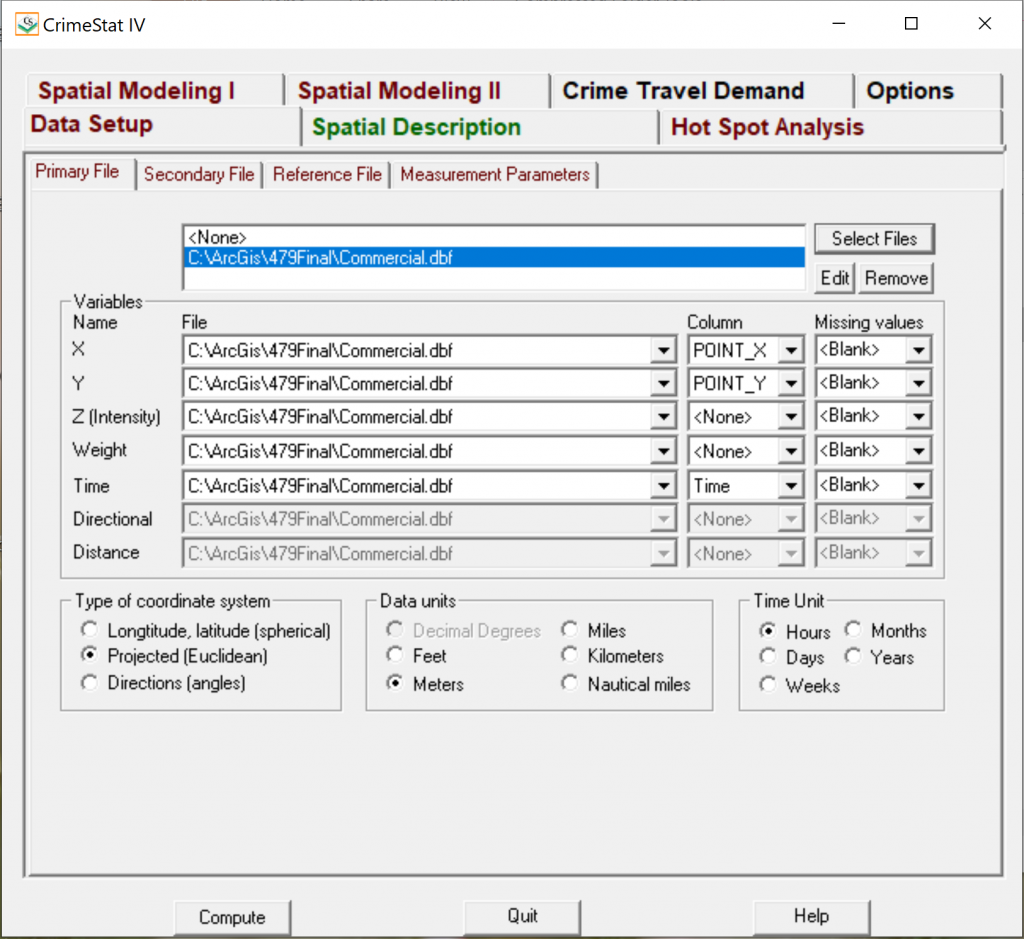
- Data Setup:
- Primary File: Conduct one at a time.
- COMMERCIAL.dbf
- RESIDENTIAL.dbf
- OUTSIDE.dbf
- Variable Names:
- X Column: POINT_X (i.e., x coordinate)
- Y Column: POINT_Y (i.e., y coordinate)
- Type of Coordinate System: Projected (Euclidean)
- Data Units: Meters
- Time Unit: Hours
- Primary File: Conduct one at a time.
- Spatial Description > Distance Analysis I:
- Nearest Neighbour Analysis (Nna): Select
- Number of Nearest Neighbours to be Computed: 50
- This number was determined after a few trial and error runs of adjusting the number (i.e., 25, 50, 75)
- Border Correction: Rectangular
- Save results as dBase ‘DBF’
- The 3 .dbf files were then opened in excel to plot the NNI graph for comparison as shown in the Results section.
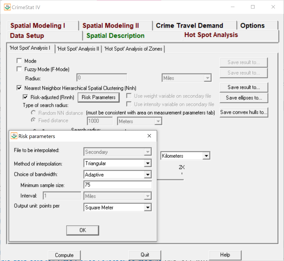
2) Nearest Neighbour Hierarchical Spatial Clustering & Risk-Adjusted Nearest Neighbour Hierarchical Spatial Clustering: The nearest neighbour hierarchical spatial clustering (Nnh) allows us to identify groups of commercial robbery incidents that are spatially close (Levine, 2013), which are shown as ellipses in our analysis. The risk-adjusted nearest neighbour hierarchical spatial clustering (Rnnh) combines the hierarchical clustering capabilities of the Nnh routine with kernel density interpolation technique (Levine, 2013). We use Rnnh to account for the fact that the population is not arranged randomly in a given region, but is, instead, concentrated in population centers.
- Data Setup:
- Primary File:
- COMMERCIAL.dbf
- Variable Names (for Primary File):
- X Column: POINT_X
- Y Column: POINT_Y
- Secondary File:
- DA_CENTROID.dbf
- Variable Names (for Secondary File):
- X Column: POINT_X
- Y Column: POINT_Y
- Z (Intensity): POP15
- Type of Coordinate System: Projected (Euclidean)
- Data Units: Meters
- Time Unit: Hours
- Primary File:
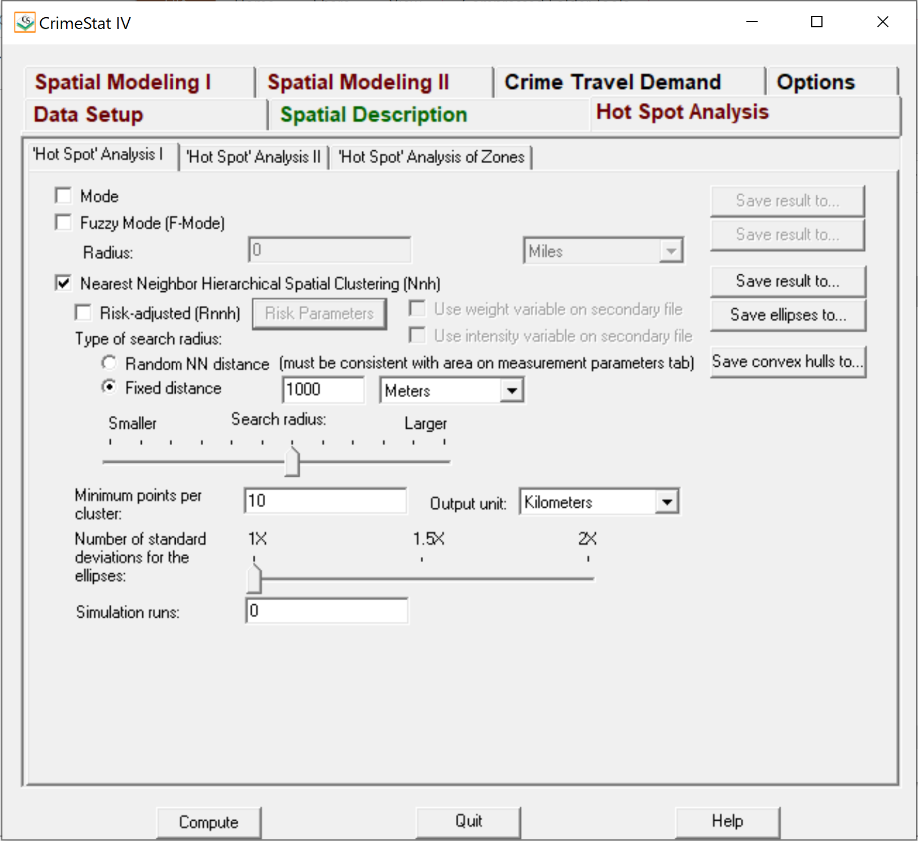
- Hot Spot Analysis > ‘Hot Spot’ Analysis I: Nnh
- Nearest Neighbour Hierarchical Spatial Clustering: Select
- Fixed Distance: 1000 meters
- Minimum Points per Cluster: 10
- Output Unit: Kilometers
- Save ellipses as ArcView ‘SHP’
- The Nnh.shp was visualized in ArcMap 10.6.1 as shown in the Results section.
- Hot Spot Analysis > ‘Hot Spot’ Analysis I: Rnnh
- Nearest Neighbour Hierarchical Spatial Clustering: Select
- Risk-Adjusted: Select
- Within Risk Parameters:
- Triangular
- Adaptive
- 75
- Square Meters
- Minimum Points per Cluster: 10
- Output Unit: Kilometers
- Save ellipses as ArcView ‘SHP’
- The Rnnh1.shp and Rnnh2.shp were visualized in ArcMap 10.6.1 as shown in the Results section.
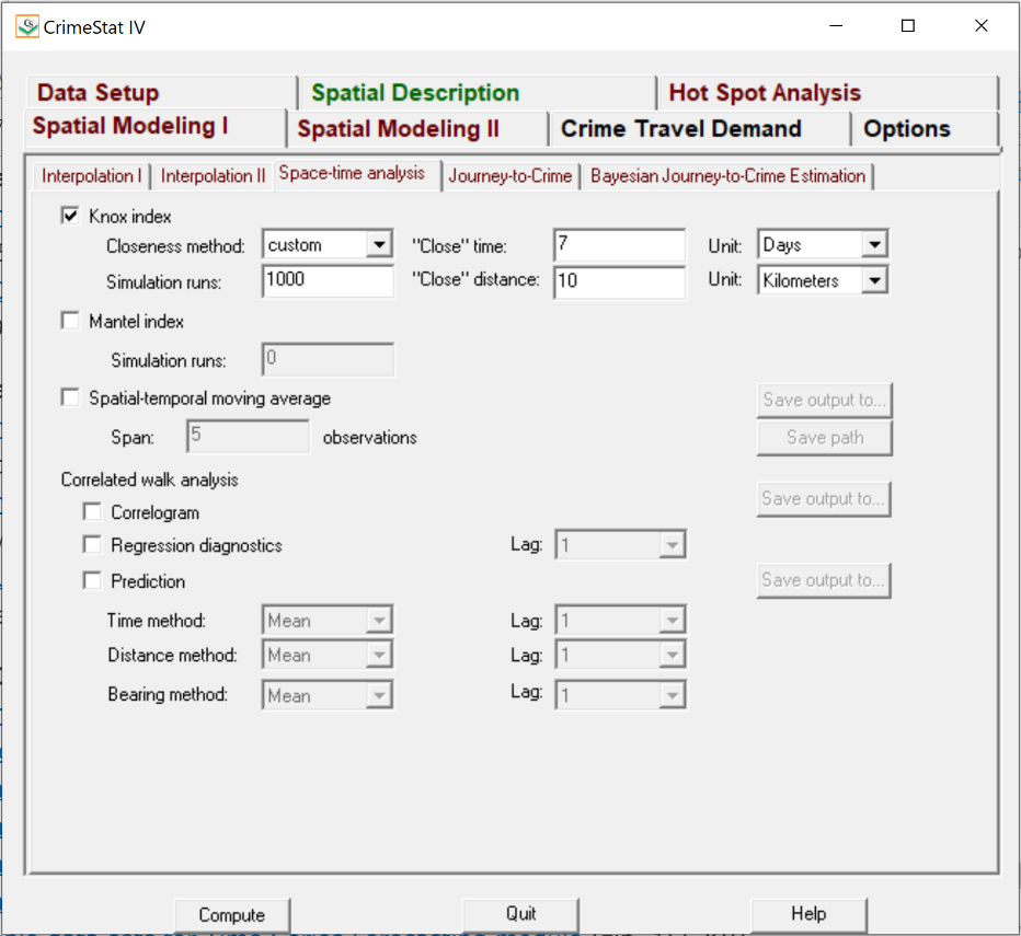
3) Knox Index: Given that crime events tend to exhibit both a spatial and temporal pattern, i.e., mimicking people’s movement throughout the hours of the day or days of the week, the Knox Index allows us to compare the relationship between incidents in terms of distance (space) and time (Levine, 2013). The distance between points are divided into close in distance and not close in distance, for which the analyst specifies what is considered close. Since ‘closeness’ is defined by the analyst, a sensitivity analysis was conducted to see how the results would vary when close distance was adjusted (i.e., 5 km, 10km, and 15km) and when close time was adjusted (i.e., hours, days, months). Note: After examining the results for adjustment of close time, we found the statistical results stayed consistent regardless of distance. As a result, we chose to rule out 5 km as it produced -1.#IND0 Chi-square values at certain percentiles while 10 km was preferred over 15 km to keep our close distance value more conservative.
- Data Setup: Adjusting close distance but not time.
- Primary File:
- COMMERCIAL.dbf
- Variable Names (for Primary File):
- X Column: POINT_X
- Y Column: POINT_Y
- Time: Time
- Type of Coordinate System: Projected (Euclidean)
- Data Units: Meters
- Time Unit: Hours
- Primary File:
- Spatial Modeling I > Space-Time Analysis:
- Knox Index: Select
- Closeness Method: Custom
- “Close” Time: 6 Hours
- “Close” Distance: Conduct one at a time.
- 5 Kilometers
- 10 Kilometers
- 15 Kilometers
- Simulation Runs: 1000
- Data Setup: Adjusting close time but not distance.
- Primary File:
- COMMERCIAL.dbf
- Variable Names (for Primary File):
- X Column: POINT_X
- Y Column: POINT_Y
- Time: Time
- Type of Coordinate System: Projected (Euclidean)
- Data Units: Meters
- Time Unit: Conduct one at a time.
- Days (when “Close” Time is set to 7 Days)
- Months (when “Close” Time is set to 6 Months)
- Primary File:
- Spatial Modeling I > Space-Time Analysis:
- Knox Index: Select
- Closeness Method: Custom
- “Close” Time: Conduct one at a time.
- 7 Days
- 6 Months
- “Close” Distance: 10 Kilometers
- “Close” Time: Conduct one at a time.
- Simulation Runs: 1000
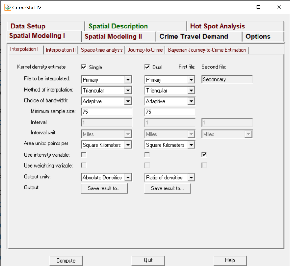
4) Single and Dual Kernel Density Estimation: Kernel density interpolation is a technique for generalizing incident locations to an entire area, which differs from the spatial distribution and hot spot statistical summaries since it generalizes those data to the entire region (Levine, 2013). Accordingly, we are able to interpolate a continuous surface of crime density (i.e., commercial robbery) based on initial data points. Single kernel density routine is applied to a distribution of a single variable (i.e., commercial robbery) while dual kernel density routine is applied to 2 distributions (i.e., commercial robbery and population aged 15 and above). As a result, the dual kernel density accounts for the population that is at risk to such criminal activities (Levine, 2013).
- Data Setup:
- Primary File:
- COMMERCIAL.dbf
- Variable Names (for Primary File):
- X Column: POINT_X
- Y Column: POINT_Y
- Secondary File:
- DA_CENTROID.dbf
- Variable Names (for Secondary File):
- X Column: POINT_X
- Y Column: POINT_Y
- Z (Intensity): POP15
- Type of Coordinate System: Projected (Euclidean)
- Data Units: Meters
- Time Unit: Hours
- Reference File:
- Primary File:
- Spatial Modeling I > Interpolation I: Single Kernel Density
- Kernel Density Estimate: Single
- File to be Interpolated: Primary
- Method of Interpolation: Triangular
- Choice of Bandwidth: Adaptive
- Minimum Sample Size: 75
- Area Units: Points per Square Kilometers
- Output Units: Absolute Densities
- Save results as ArcView ‘SHP’
- The KD_Single.shp was visualized in ArcMap 10.6.1 as shown in the Results section.
- Spatial Modeling I > Interpolation I: Dual Kernel Density
- Kernel Density Estimate: Dual
- File to be Interpolated: Primary
- Second File: Secondary
- Method of Interpolation: Triangular
- Choice of Bandwidth: Adaptive
- Minimum Sample Size: 75
- Area Units: Points per Square Kilometers
- Use Intensity Variable (for Second File): Select
- Output Units: Ratio of Densities
- Save results as ArcView ‘SHP’
- The KD_Dual.shp was visualized in ArcMap 10.6.1 as shown in the Results section.
ArcMap 10.6.1:
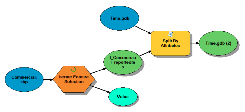
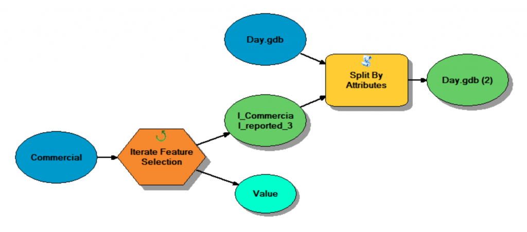
1) Kernel Density Estimations for Days of the Week and Months in a Year: Kernel density estimations for days of the week and months in a year were conducted in ArcMap 10.6.1, instead of CrimeStat, as it required repetitive steps that could be performed more efficiently by building geoprocessing workflows using ModelBuilder. The workflow is outlined in Figure 2 while Models 1 to 4 are the models used to conduct this operation. As a result, a total of 19 kernel density surfaces (i.e., 12 months and 7 days) were created.
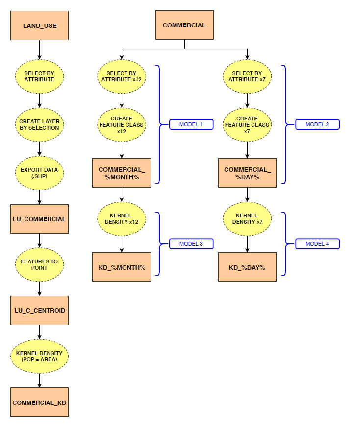
Figure 2. Flowchart showing data and process used to create kernel density estimates in ArcMap 10.6.1.
Model 1. Select by Attributes (i.e., each month) to create a point feature class in a geodatabase.
Model 2. Select by Attributes (i.e., each day) to create a point feature class in a geodatabase.

Model 3. Months point feature class to kernel density surfaces.
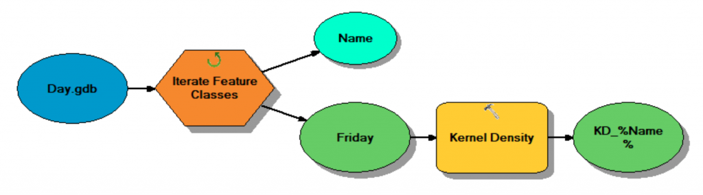
Model 4. Days point feature class to kernel density surfaces.
2) Visualization: Shapefiles created from CrimeStat (i.e., Nnh.shp, Rnnh1.shp, Rnnh2.shp, KD_Single.shp, and KD_Dual.shp), along with the kernel density surfaces created within ArcMap 10.6.1, were all visualized as maps. Note: Most maps were visualized with the light gray canvas Esri basemap.