Nearest Neighbour Analysis:
The nearest neighbour index tests whether the average nearest neighbour distance is significantly different that what would be expected on the basis of chance (Levine, 2013). Patterns are used to discern clustering or dispersion of a phenomenon; values closer to 1 indicate dispersion, values closer to 0 indicate clustering. First order crimes exhibit the most clustering behaviour, as shown by the steeper peak in Figure 1 (applicable for all robbery types). The two variables are positively correlated: increasing the index increases the order. The nearest neighbour index varies according to crime type, from lowest to highest: commercial, outside, residential. The indices are most significant until approximately the 14th order, which was the cutoff point for ranking the indices. The large Z-score, absval(-104.2955), and small p-value of 0.0001 indicate statistical significance. High aggregative tendencies of commercial robberies could be due to the proximity of business, as well as city zoning laws. Furthermore, crime intensity is suspected to be higher for areas with lots of neighbours, like the facilities in a shopping mall. Increasing the order increases distance, so the neighbours become “coarser” at this scale; the neighbours are the malls themselves as opposed to the stores within them. The “levelling off” observed in our plots after the 14th order is a function of the increasing distance between neighbours.
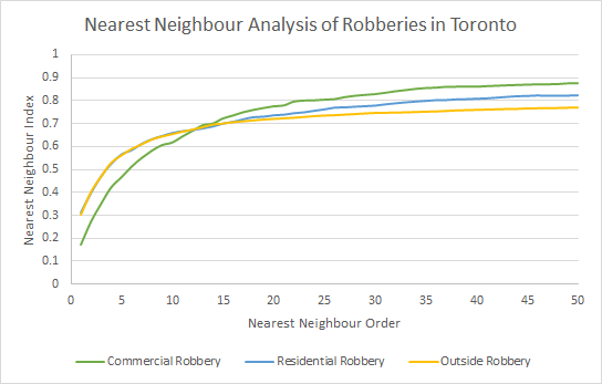 Figure 1. Nearest neighbour index by types of robbery.
Nearest Neighbour Hierarchical Spatial Clustering & Risk-Adjusted Nearest Neighbour Hierarchical Spatial Clustering:
Nearest neighbour hierarchical (Nnh) spatial clustering displays hot spots based on a defined minimum radius, 1 km for this analysis (Levine, 2013). Hot spots are depict locations with the most incidents (Levine, 2013) and the agglomerative clustering method used merges clusters in increasing order. The nearest neighbour ellipses in the risk-adjusted analysis map are drawn only by crime frequency. Crime aggregates near the downtown core and decreased outwards. However, this clustering routine does not account for underlying population so we cannot be certain about whether the ‘hot spot’ in Downtown Toronto is a consequence of the high population residing there. High crime frequency in a densely populated region proves less significant than high crime frequency in a sparsely populated region. Risk-adjusted analysis normalizes crime frequency by population aged 15 and above, allowing us to consider the underlying population per dissemination area (Map 1). The population-adjusted clusters represent crime intensity and population intensity. The previously mentioned Nnh method merely clusters points within a distance threshold, held constant throughout the study region. Risk-adjusted nearest neighbour hierarchical spatial clustering (Rnnh) identifies risk instead of crime volume (Levine, 2013). Rnnh utilizes a base variable (population over the age of 15) and adjusts the distance threshold accordingly. First order ellipses utilize the centres of population adjusted of population adjusted clusters to aggregate larger ones. Rnnh allows us to identify high risk crime regions instead of high volume crime regions; high volume does not necessarily imply high risk if there was equally large underlying population.
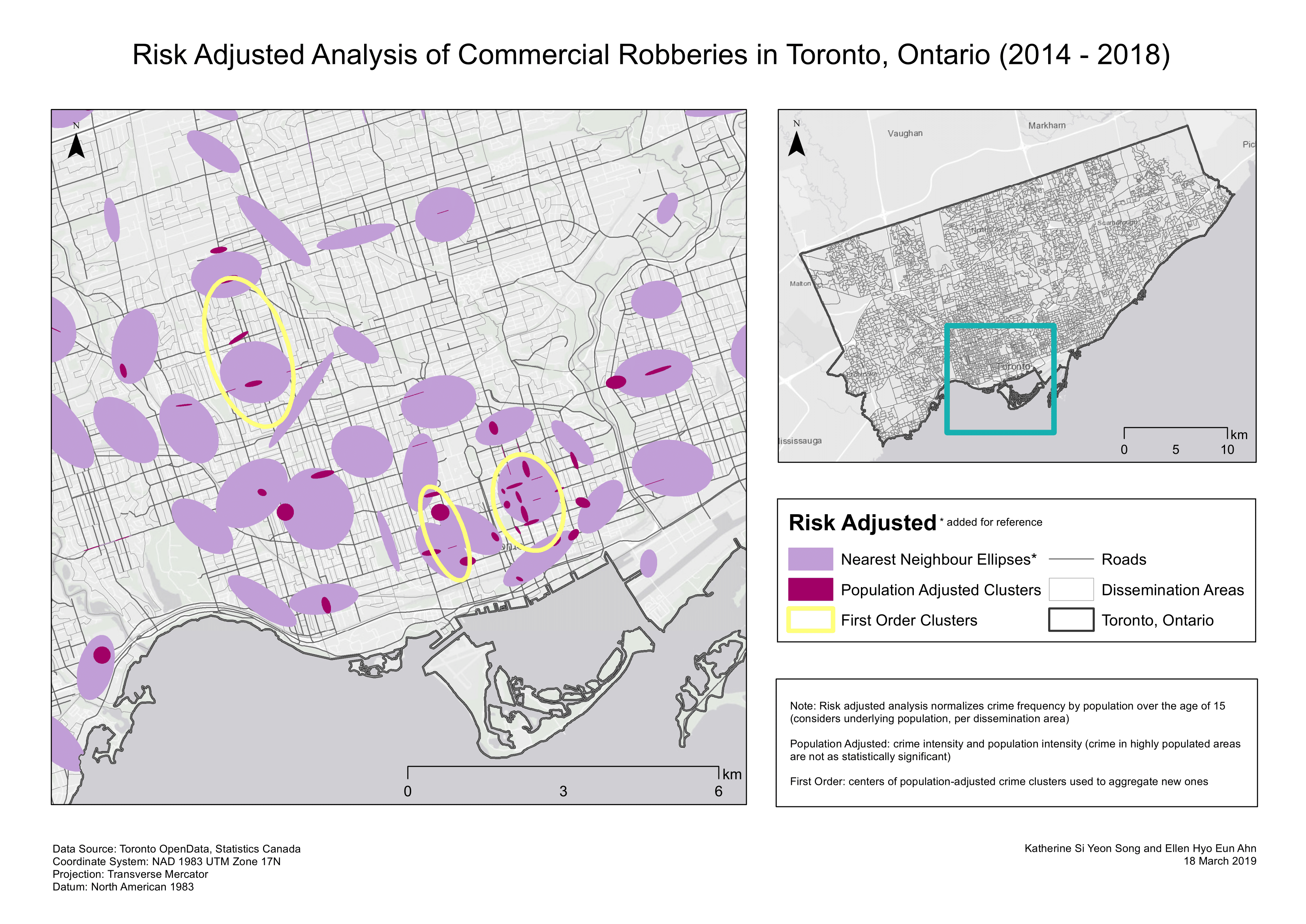
Map 1. Risk-adjusted nearest neighbour hierarchical spatial clustering.
Knox Index:
The Knox index compares the relationship between incidents through time and space (Levine, 2013). Pairs of recorded commercial robberies are compared by distance and by time; point pairs are measured by closeness and non-closeness. More concisely, incidents that are close in space or not close in space and incidents that are close in time or not close in time. In the context of our commercial robbery dataset, temporal patterns across hours of the day, days of the week, and months of the year were analyzed. ‘Closeness’ was compared for pairs of data values and compared to the expected number of pairs if there were no existing relationship between space and time in the data (null hypothesis). Month, day, and hour indices produced statistically significant results in terms of the Chi-square statistic (most up to the 97.5th percentile), allowing us to reject the null hypothesis regarding a random distribution between space and time. The Chi-square statistic is the difference between the observed and expected values. In our analysis, we observed more commercial robberies close in space and in time than expected, where close in time entails 6 hours, 6 months or 7 days and close in space entails 10 km proximity. There were more commercial robberies observed not close in time and not close in space than expected, less commercial robberies observed close in space but not close in time than expected, and less commercial robberies observed close in time but not close in space than expected.
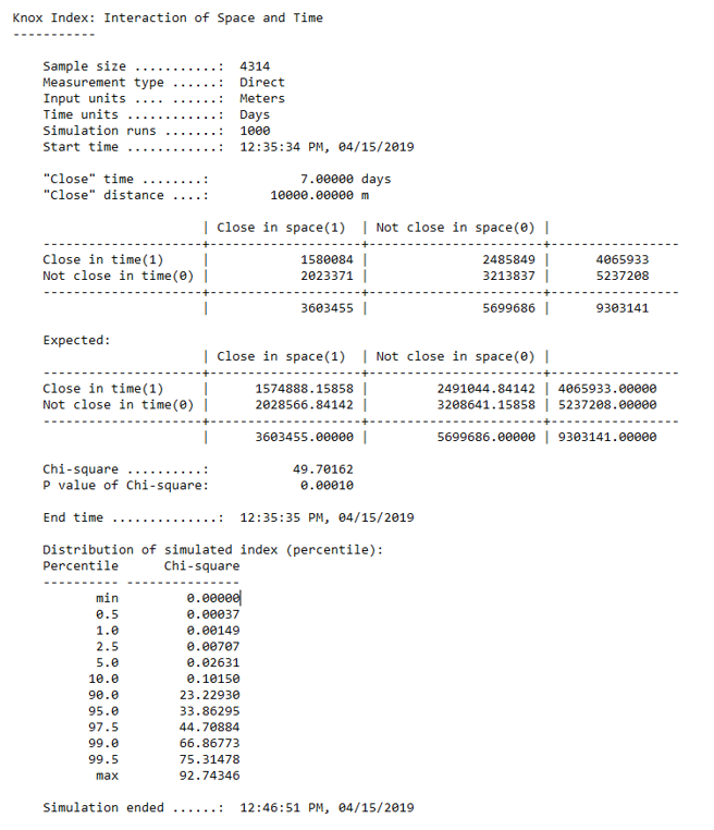 Figure 2. Output results from one of our tests, with ‘close’ distance at 10 km and
‘close’ time at 7 days.
Kernel Density:
Kernel density estimations (KDE) create surfaces that generalize crime incidents to a specific location (Conlen, n.d.). KDE is calculated using the weighted distance of every data point for a specific location. The estimate becomes higher or lower depending on the probability of seeing a point (like a commercial robbery) at that location. Bandwidth effects has an affect on kernel shape; lower bandwidths preclude the contribution of distant points. We used an adaptive bandwidth and a minimum sample size of 75. The adaptive bandwidth option allocates smaller bandwidths to regions with higher point concentrations (more commercial robberies) to provide more consistent statistical estimates (Levine, 2013). Crimestat’s single kernel density routine is applied to point locations, like crime incidents. The primary file (i.e., commercial robbery) is interpolated to display the number of incidents occurring per grid cell, representing crime volume (Map 2). The dual kernel density routine is (somewhat) comparable to the risk-adjusted analysis; population is used as a secondary variable and we are now identifying high risk areas for commercial robberies based on regions of higher crime intensity (Map 3). We observed crime spots throughout the city, with a notable “cold” spot near Scarborough in the single density surface. The dual density surface provided more ‘enlightening’ information, with a hot spot near a locale in close proximity to Casino Woodbine. This corroborates the findings of Bernasco, Ruiter, and Block (2017) that robbers do prefer cash-intensive facilities. The same “cold” spot was found near Scarborough and some prevalence of hot spots surrounding the downtown area.
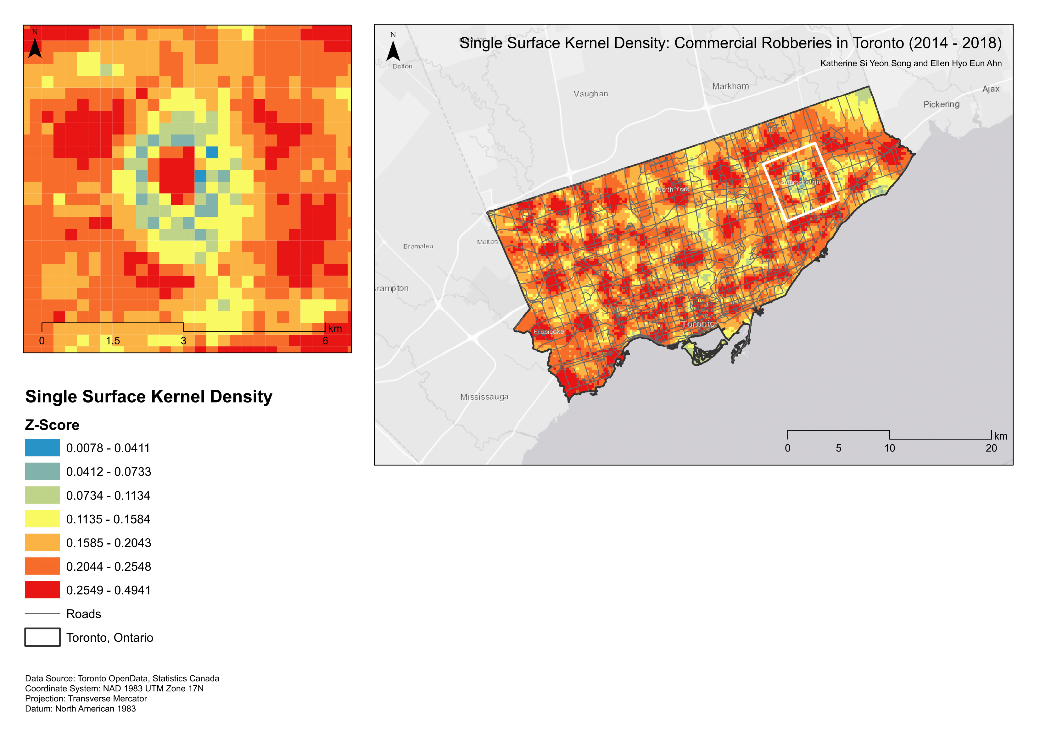
Map 2. Single kernel density surface.
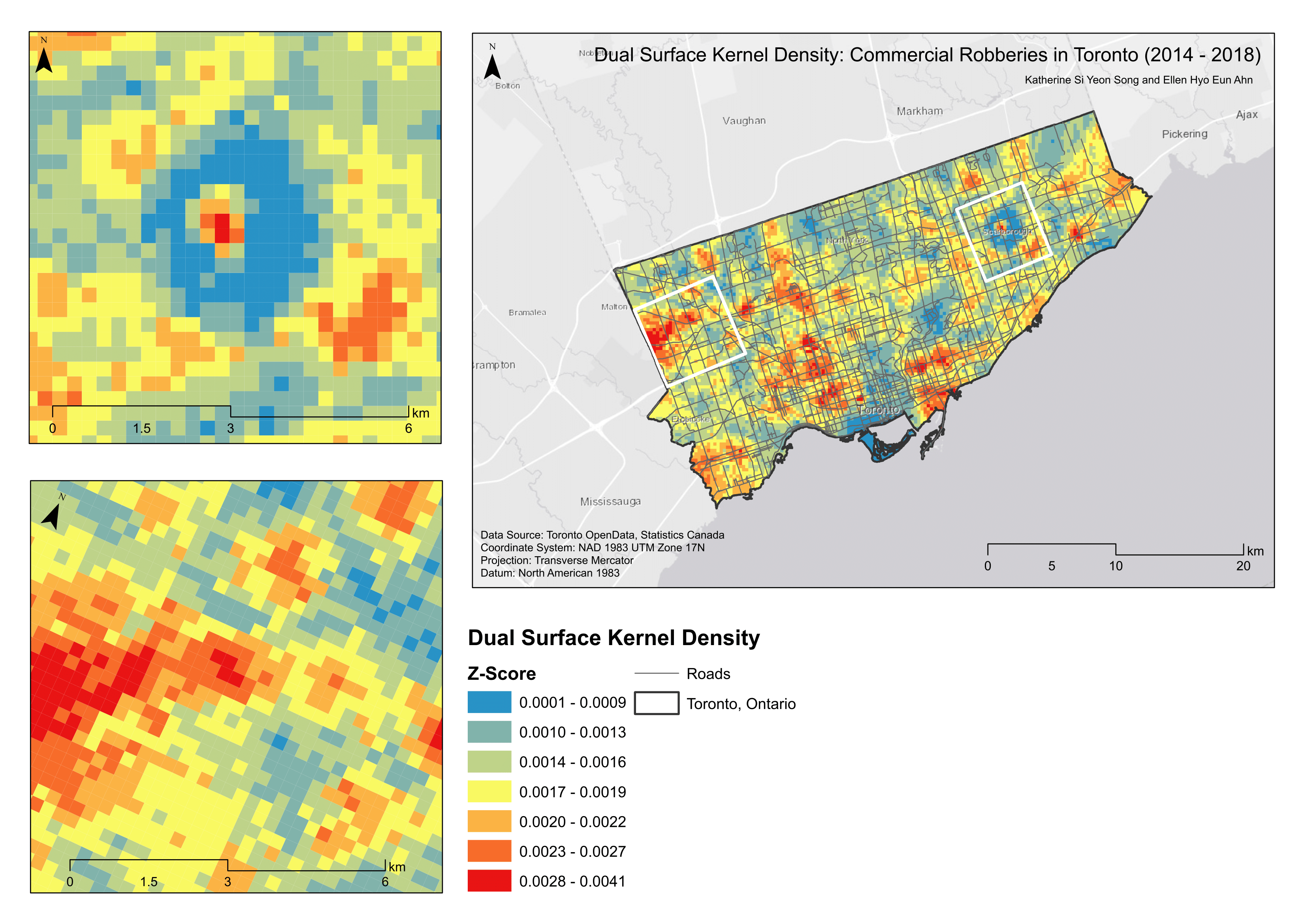
Map 3. Dual kernel density surface.
Temporal kernel density surfaces to analyze patterns between days of the week and months of the year were also generated (Map 4 and 5). From the density surfaces generated in this analysis, our findings suggest that the location preferences of robbers remain relatively stable over time. These findings vindicate those of Bernasco et al. (2017), implying that robbers indeed prefer cash-intensive businesses and facilities associated with high benefit and low risk. Their findings entail unwavering preference for certain businesses, even when they are closed and activity levels are low. Facilities attracting robberies tend to do so throughout the day with little variation by hour as well as throughout the week without much variation by day. Crime, and more specifically robbery, in Toronto generally seems to aggregate near the downtown area. Andreson and Malleson’s (2016) study on crime seasonality in Vancouver suggests that crimes like robbery appear to “occur in the same places regardless of the season of the year,” perhaps legitimizing the ‘unenlightening’ results of the 12 month kernel density surfaces. Lastly, we examined a dual kernel density surface for commercial land use (with each polygon converted to centroids), with area in the population field, but saw no relationship between commercial land use area and observed crime spots in our kernel density surfaces. We chose not to include a map of this surface as it provided no additional benefit when visualized (than what was already explained) as the surface is very smooth with no extreme density values throughout the entire surface for the City of Toronto.
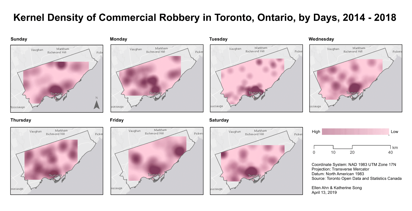
Map 4. Kernel density surfaces by days of the week.
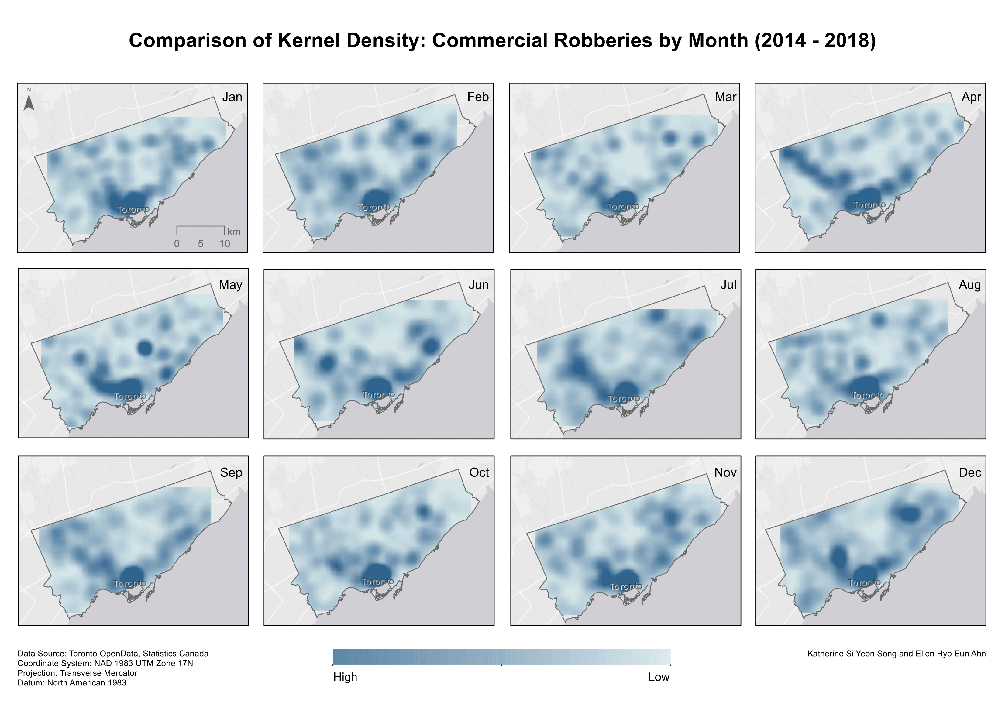
Map 5. Kernel density surfaces by months of the year.