I: PREAMBLE

In my last post, I tried to establish some reasons as to why there were cross-shaped artifacts in the 2D roughness algorithm I had been using. One thought that came to mind after writing that: why should there be a bias towards one point within a local neighbourhood? As Shepard (2003) states, one can implement ‘interleaving’ in order to maximize the information used.

Interleaving can be best understood by beginning with a one-dimensional example. For instance, assume that we have a profile 1m long, and wish to measure roughness (calculate RMS Slope and Hurst Exponent) over scales (step-sizes) of 1-5cm. For Δd=1cm step-sizes, points to be sampled in the calculation would then be [0, 1, 2, … , 100] cm; those for Δd=2cm step-sizes would be [0, 2, 4, … , 100] cm; and so forth. For small step-sizes, we are obtaining not only a relatively large number of samples (ie. 100 for Δd=1cm) – but all possible samples for points separated by 1cm. However, consider Δd=5cm, the largest step-size in this investigation, for which the sample points would be [0, 5, 10, … , 100] cm. However, what about sample pairs such as (1, 6)cm, or (2, 7)cm, or (88,93)cm? Such pairs would not be included in the conventional approach, which I shall denote ‘non-interleaved’.

In this case then, interleaving would increase the number of available sample pairs by a factor of 4 (ie. allowing for the inclusion of the sets of pairs [1, 6, 11, … , 96] cm; [2, 7, 12, … , 97] cm; [3, 8, 13, … , 98] cm; and [4, 9, 14, … , 99] cm).  This is not without caveats – particularly, as Shepard points out, the fact that the increase in information available owing to interleaving is not as large as it may appear, owing from the fact that adjacent points are likely to be significantly correlated with one another.

In 2 dimensions, the extra information available from interleaving is even greater, owing from the larger number of combinations given the higher dimensionality. This is apparent upon visually comparing the non-interleaved vs. interleaved roughness algorithms.

In order to understand the benefits of interleaving in 2D, it is helpful to review the non-interleaved 2D roughness algorithm.

First,, all lag vectors emanate (radially) from the central pixel (black square) within a neighbourhood. To calculate the RMS Deviation for a given value of Δd (step-size), the SSDH (sum of squared differences in heights) between points on each and every ‘arm’ is calculated (ie. for (i) and (ii), 4 lines are integrated together, while for (iii), 8 lines are). This value is then divided by the number of sample pairs, and the square root taken, resulting in the RMS slope value at the central pixel, for a given value of Δd. This value is plotted as a single point on a variogram, after which the Δd value is iteratively changed (both in terms of magnitude and direction). Once Δd values have been obtained throughout the size scale desired, a line of best-fit is applied to the variogram in order to determine the RMS Slope and Hurst Exponent – again both these being representative for only a single pixel. The entire process is necessarily repeated if one desires to produce a roughness map of a 2D region.

(This procedure is outlined in greater detail here.)

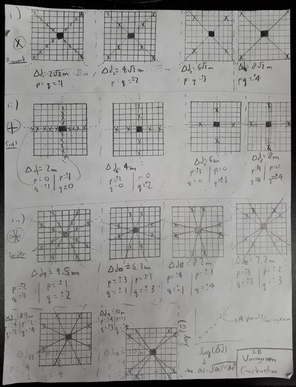
The rub is that, as with the 1D case, this non-interleaved algorithm is biased towards a single point (in this case the central pixel). But how can we do this in a computationally feasible manner? The obvious choice would be to just apply the non-interleaved algorithm, but iterating over every point within the central pixel’s neighbourhood. While this would be comprehensive, this would entail (approximately) that, given a standard 17×17 neighbourhood size, the algorithm’s computation time would increase by a factor of 189. When it already requires ~8 hours for the Highway Flow DEM (2700×2700 pixels), however, this quickly appears ridiculous, as such an algorithm would therefore require ~2 months of computation time.

 

___________________________________________________

II: PROPOSED METHOD  

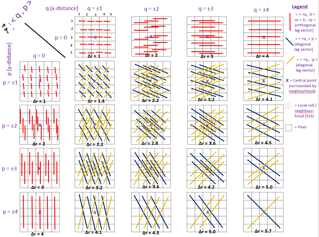
Fortunately, another method can be envisaged, outlined in detail here, and visualized below. The primary and essential difference between the previous algorithm and the new one is that, like for the analogous 1D case, every possible combination of points separated by a lag vector (now two-dimensional, rather than one) contributes to the calculation, rather than only a fraction of such. No longer do the combinations selected consist merely of the subset of those connected to the central point; now, all connections/points within the neighbourhood are considered.

Methodologically, once the Gaussian high pass filter has been applied to the DEM (denoted the HPF-DEM), the algorithm works iteratively to find the RMS Deviation associated with each value of the lag vector r = <q, p>, as the pseudo-code below will attempt to show.

 

FOR the ith row of the HPF-DEM

FOR the jth column of the HPF-DEM

        –> Define a neighbourhood centred on the (j,i)th pixel of the HPF-DEM, given a user-defined neighbourhood radius 

        FOR each value of step-size p in the y-direction, ranging from [0, ±1, … , ±4*]

            FOR each value of step-size q in the x-direction, ranging from [0, ±1, … , ±4*]

                IF the lag vector is parallel to the grid (eg. <4,0> or <0,1>) 

                      –> Find the  heights associated with the points separated horizontally by the lag vector <+q, +p> (ie. red lines in diagram), and determine the RMS Deviation amongst them, corresponding to all of the red lines within a given grid below

 

                ELSE the lag vector is not parallel to the grid (eg. <4,2> or <1,4>) 

                     –> Find the  heights associated with the points separated horizontally by the lag vector <+q, +p> (ie. blue lines in diagram), and determine the RMS Deviation amongst  them, corresponding to all of the blue lines within a given grid below

                     –> Find the  heights associated with the points separated horizontally by the lag vector <+q, -p> (ie. yellow lines in diagram), and determine the RMS Deviation amongst them, corresponding to all of the yellow lines within a given grid below 

                END

 

            END

        END

        –> Having calculated all of the RMS Deviations associated with all of the combinations of lag vectors for a given central point (within its neighbourhood), construct a variogram and employ weighted** linear least-squares fitting to determine the line of best fit, and hence the RMS Slope and Hurst Exponent associated with this central point. 

END

END

 

* Note that the maximum orthogonal step-size in this example is 4, matching the visualization (for which the largest lag vector is (±4, ±4)).

** In a normal (non-weighted) least squares fit, all points are accorded equal weighting in the determination of the line of best fit. However, when considering the interleaving algorithm, it is apparent that the RMS Deviations for some lag vectors should be given more weight than others. For instance, the RMS deviation for the lag vector <+1, +1> is calculated from many more point pairs than that for the lag vector <+4, +4> (16 point pairs vs. 1, respectively, to be precise). A simple/intuitive modification is thus to weight the point representing the RMS deviation at <+1, +1> on the variogram by a factor of 16 greater than the point representing the RMS deviation at <+4, 4> – and likewise to employ proportional weighting in this manner for all points. The current algorithm employs this modified least-square fitting – I would appreciate thoughts on whether this procedure is valid.

 

Let’s put this algorithm now into the context of an actual DEM. At a single pixel within this DEM, we can for instance set a local neighbourhood radius of 2 pixels, producing a 5×5 pixel neighbourhood centred about our pixel of interest. Everything I now describe therefore takes place within the bolded inner loops in the algorithm above. Now, we should technically start with p=q=0, for which the lag vector would be <0, 0>. However, since this would just be the difference between the height of a point with itself, this isn’t physically meaningful to us. Thus, our first non-trivial lag vector is <±1, 0> (ie. q = ±1, p = 0), for which the connections within the local neighbourhood can be seen on the 5×5 grid to the top-left of the diagram. The ± sign lies in the directional interchangeability of the lag vector: for instance, it could be <+1, 0>, moving from (1, 1)–>(2, 1), or equivalently <-1, 0>, moving from (2, 1)–>(1, 1). Over the whole neighbourhood, this particular lag vector therefore has 16 connections, for which an RMS Deviation will be calculated for a lag distance of Δr = 1 (in units of  pixels). Then, the same process is repeated for the lag vector <±2, 0>, then <±3, 0>, then <±4,0>, each time producing one value of RMS Deviation, corresponding to lag distances of Δr = 2, 3, and 4, respectively.

Next, we’ll iterate from p=0 to p=±1, resetting q back to q=0, calculate an RMS Deviation, then iterate q to ±1, ±2, ±3, and ±4, as before. However, upon getting to p=q=±1, we will encounter an additional consideration; the fact that p=±1 and q=±1 produce 2 distinct lag vectors (in terms of direction): <+1,+1> and <+1,-1> (or equivalently, <-1,-1> and <-1,+1>). While the previous algorithm would have combined both of these connections to produce one RMS Deviation value, on the basis of both vectors having the same magnitude (sqrt(2)~=1.4), I believe their is value in leaving them separated, in light of anisotropy considerations (this is further apparent in the variograms I produce in a subsequent section). As a result, the lag combination p=q=±1 produces 2 distinct RMS deviation values for the same step-size Δd on the variogram. In fact, any lag non-orthogonal lag vector with p≠q (eg. p=±2 and q=±1) would have 4 distinct RMS deviation values for a single value of Δd, due to the fact that both lag vectors <±2,±1> and <±1,±2> share the same magnitude of sqrt(5).

 

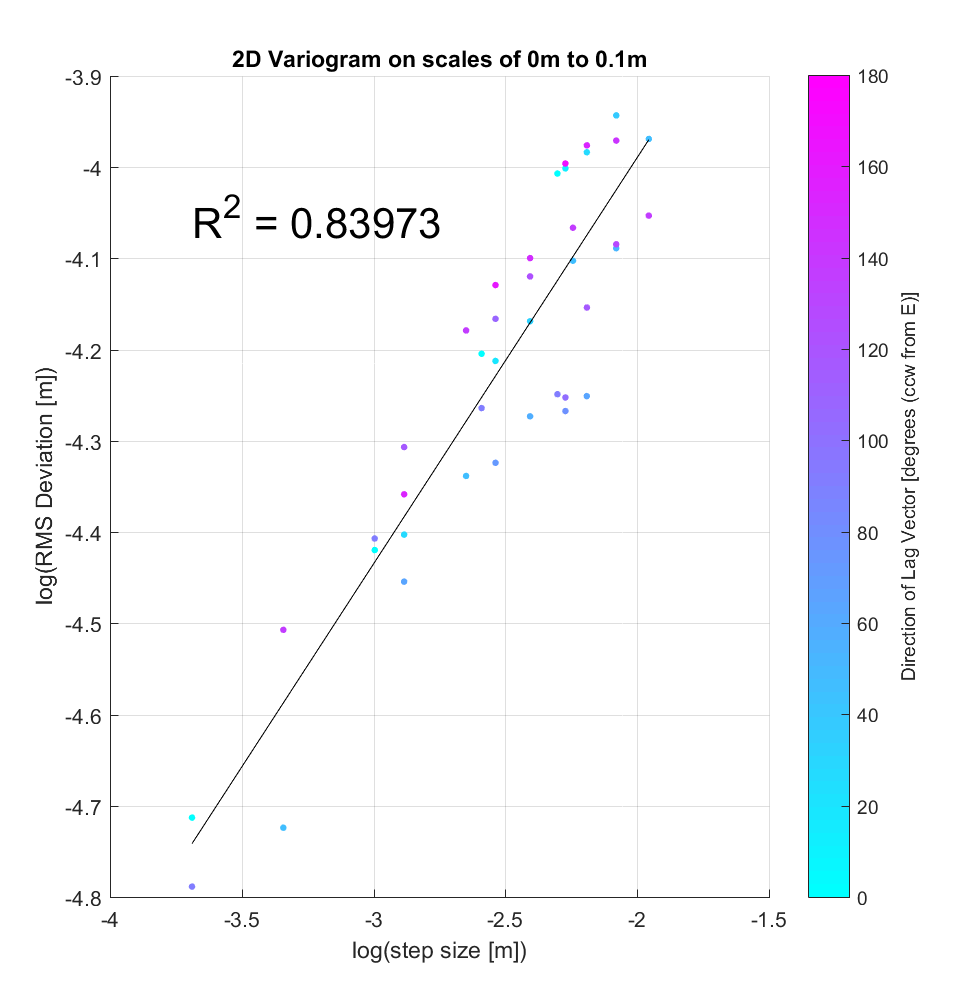
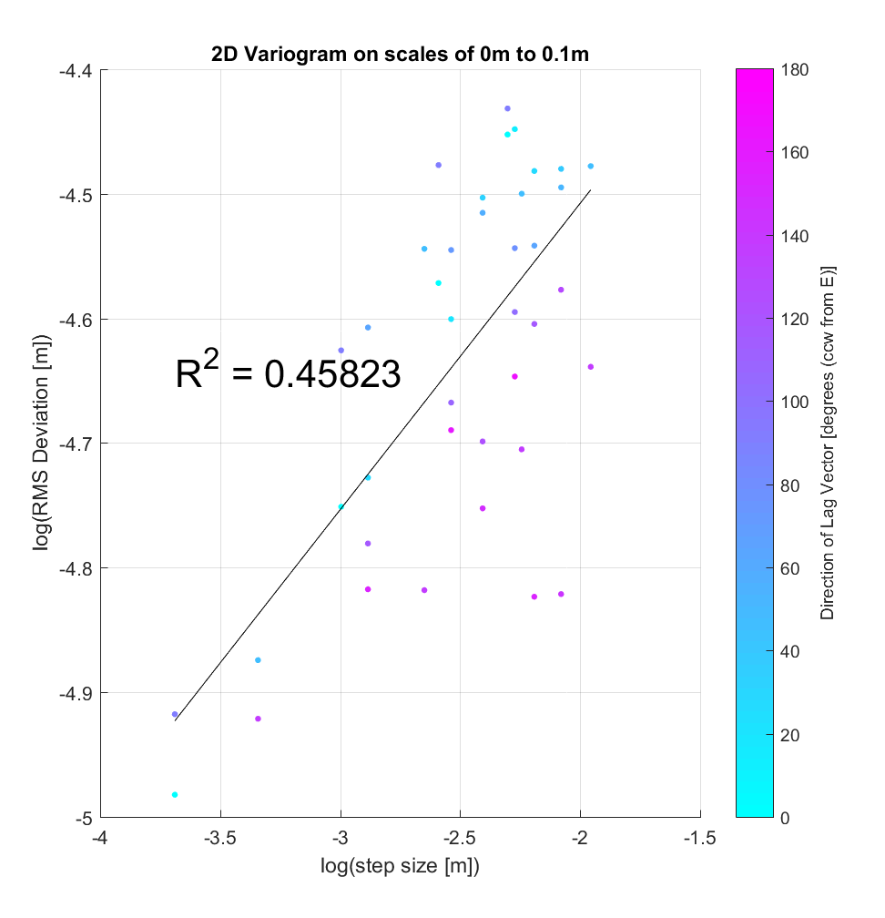
Shown below is an example of a variogram that could be produced via the application of this algorithm to a DEM. As described above, it is evident that for any given step-size, there are either 2 or 4 associated RMS Deviation values, representing the 2 or 4 different directions of the lag vectors with that step-size. It’s evident that another benefit of calculating distinct RMS Deviation values for each direction is that we can qualitatively examine the anisotropy of a surface, by associating a colour with each point on the variogram, where the colour is proportional to the angle of the lag vector associated to a given point. Indeed, this sample variogram shows a slight bias of smaller-angle lags (blue points) to lower RMS Deviation values, and conversely larger-angle lags (purple points) to higher RMS Deviation values, implying a degree of anisotropy. I wonder whether further efforts to try to quantify this effect are of interest to us?

 

___________________________________________________

III: PRELIMINARY RESULTS 

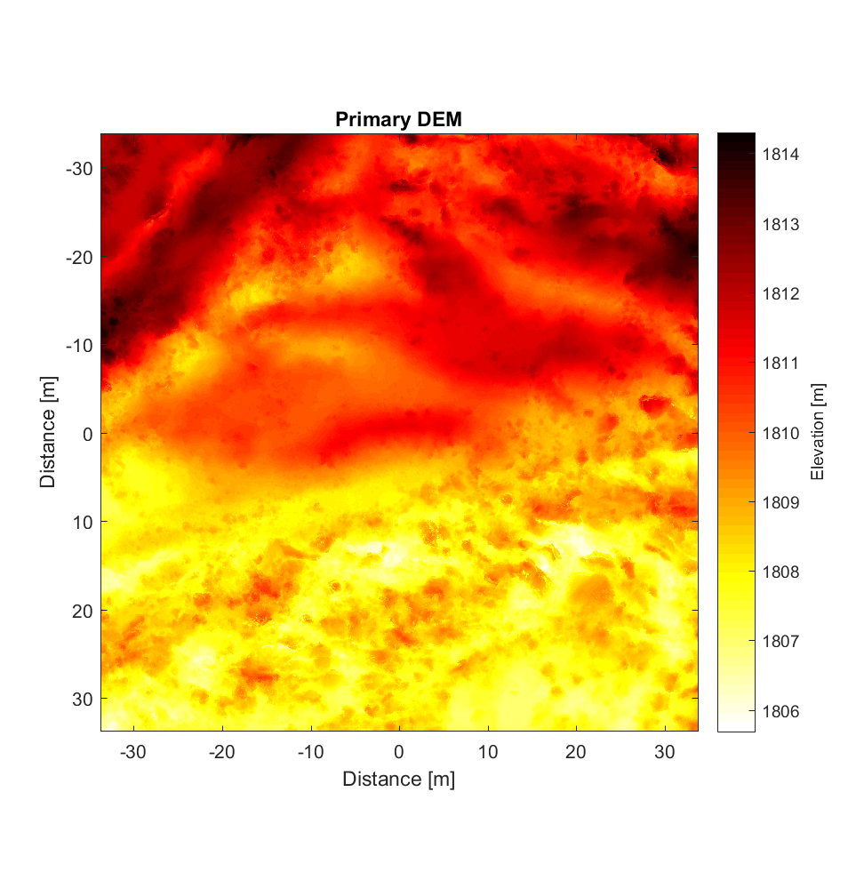
Mike provided me with a LiDAR DEM (2.5cm/pixel resolution) from Highway Flow before he left, of which I extracted a 2700×2700 block for roughness analysis. The results upon application of the new, interleaved 2D roughness algorithm are below, for a neighbourhood size of 11×11 and high-pass Gaussian filter cut-off wavelength of 50m. To my surprise (and relief), the new interleaved algorithm required less time than the non-interleaved version (for the same DEM), requiring only 6h vs. the previous 8h. I’m particularly surprised because this version has more nested loops, in addition to its having to perform far more calculations per pixel. (However, for larger neighbourhood sizes, the number of calculations, and computation time required, correspondingly, does become prohibitive; the 400×400 variograms shown at the end require ~1 billion calculations per pixel).

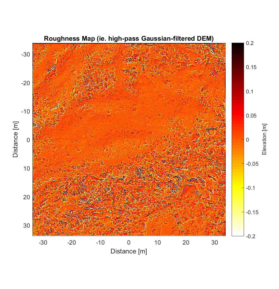
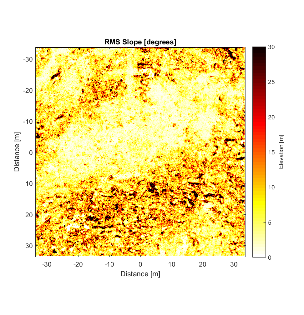
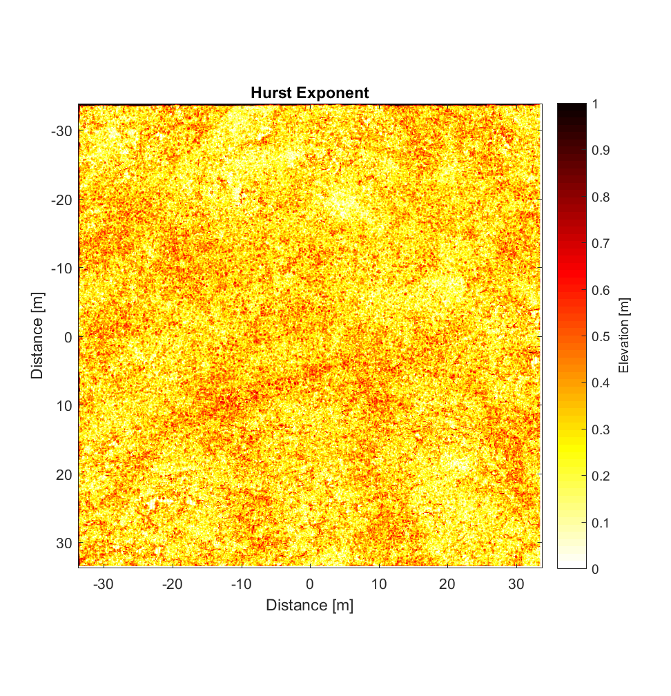
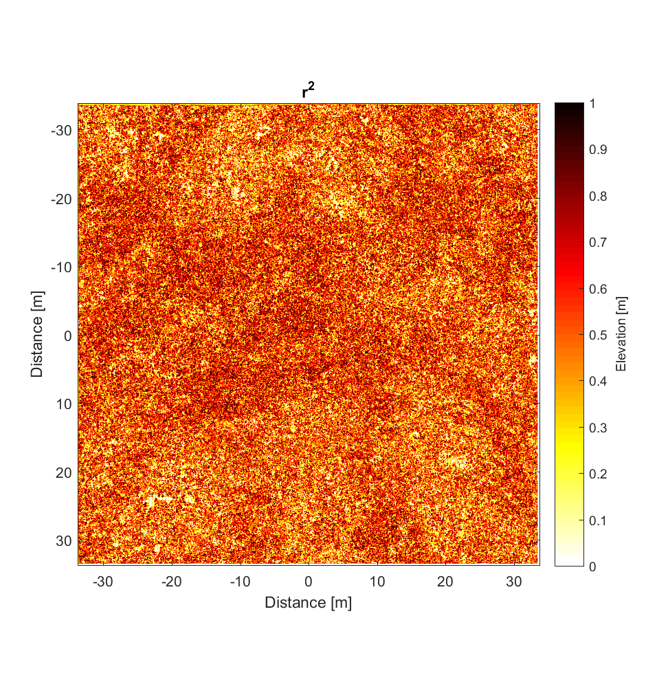
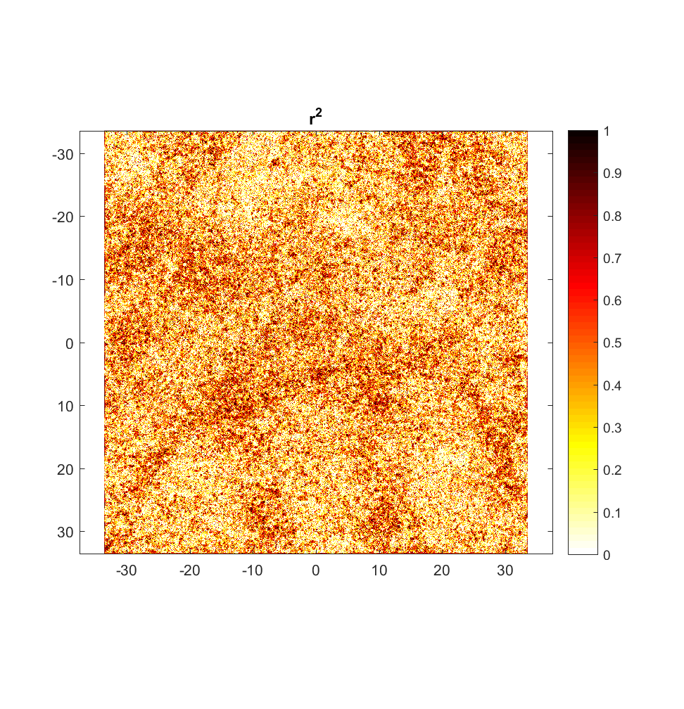
The RMS Slope and Hurst Exponent maps are similar to the roughness maps obtained using the non-interleaved algorithm. However, the higher r^2 values are a significant improvement (compare to plot below), albeit showing the same general pattern.

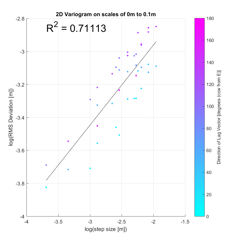
Meanwhile, the variograms (ones from sample locations shown below), while having improved r^2 values in general, illustrate significant anisotropy, with blue points clustering amongst other blue points (small angle), and purple with purple (large angle). One could imagine segregating each variogram into 2 subsets with respect to angle, producing 2 lines of best fit with similar slope and differing y-intercept. Physically, the character of anisotropy at these locations implies that primarily influences RMS slope (y-intercept), but not Hurst Exponent (slope). A more systematic analysis of all variograms throughout the Highway Flow DEM would perhaps elucidate and more precisely quantify these anisotropic roughness effects.

Note that these variograms are representative of roughness scaling relationships only over the very limited and small-scale range of 2.5-14 cm.

 

 

 

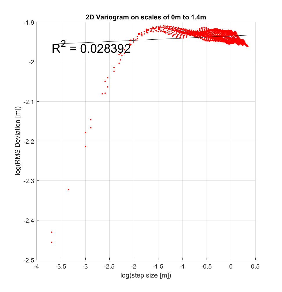
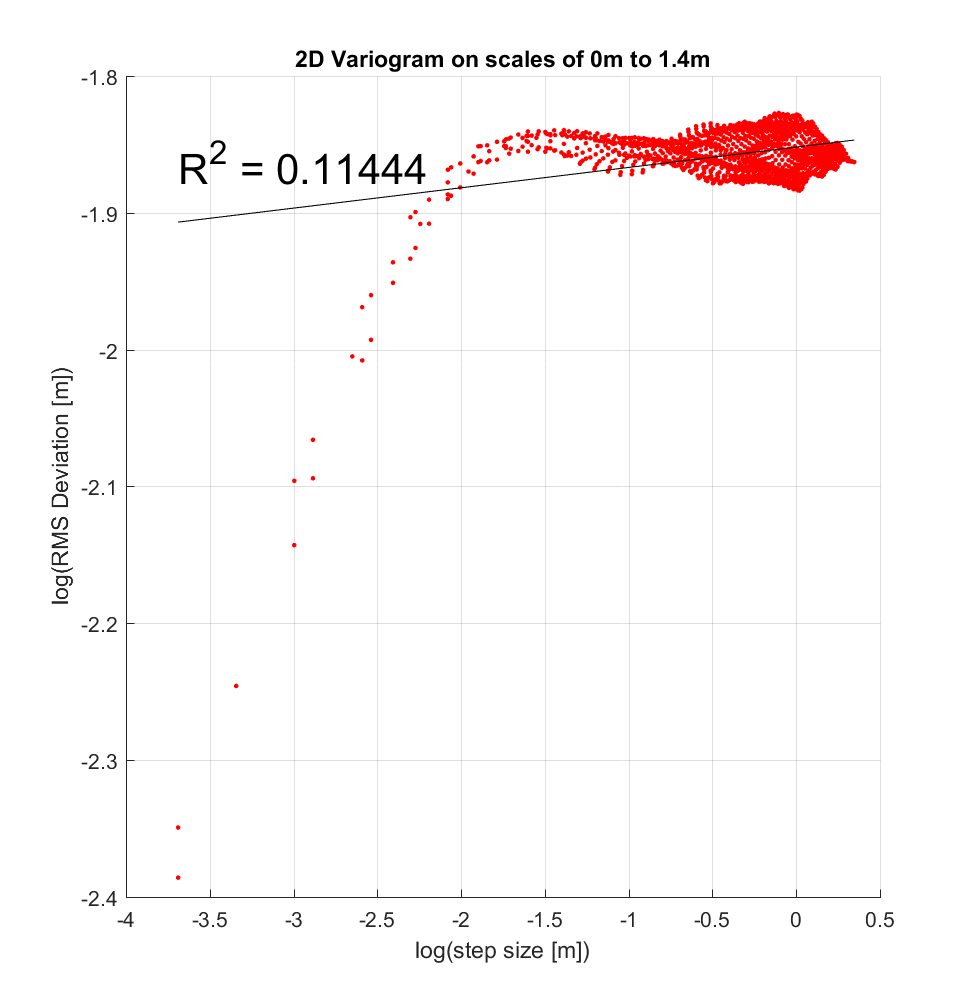
I also chose to perform the interleaved roughness algorithm with a very large neighbourhood size of 400×400 (ie. 10×10 m), since a similar range of scales was employed at COTM in Neish et. al. (2017), which employed a maximum variogram scale of 12m. Resulting variograms at 2 sample locations suggest a breakpoint at approximately log(-2 m), or ~14cm, though the concept of a ‘breakpoint’ for this case is rather imprecise, given the gradual change in slope observed at and above this scale. Moreover, over the range of log(-3.7 m) to log(-1.5 m), or 2.5 to 22cm, the changing slope would perhaps better be bit by a polynomial, such as a quadratic, as was employed by Shepard (2003) in Figure 3b. Figure 3b also featured a maximum RMS Deviation value, which appears to likewise be the case here as well, where the maximum RMS Deviation here is log(-1.9 m) or log(-1.825m), or 15-16 cm.

As for next steps, I could apply the interleaved roughness algorithm to other DEM’s at COTM (Mike says there are upwards of 30 others), and similarly determine whether they have similar breakpoints and/or values of RMS Slope and Hurst Exponent. Mike also recommended that I compute Hurst exponent using more conventional methods for the determination of fractal dimension (such as the box-counting method), and see if the results are comparable to the Hurst exponent determined by variogram analysis such as that employed here.