Excel Basics
- Open a blank Excel spreadsheet
- Type 2 in cell A1. Next, go to cell C2 and type =A1 and hit Return. The result is that cell C2 contains the number 2.
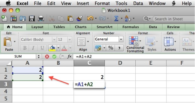
- We can use formulas to perform simple math. Type 2 in cell A2. Next, go to cell C3 and type =A1+A2 and hit Return. Notice that cell C3 contains the number 4
- Replace the addition ( + ) symbol with the minus ( – ) symbol and the result is 0. Replace with the multiplication symbol ( * – asterisk) and the division symbol ( / – forward slash) to see more results.
- You can also use this to perform more complicated math. If you want to calculate a percentage click on cell C4 and type =A2/A1*100 and the result is 100. This translates to =smaller number/larger number *100 (to move the decimal two places).
Change the value of cell A1 to 4 and the result in cell C4 updates to 50. All the previous formulas update as well.
Percent change is a very useful formula to know.
- Click on cell C5 and type =(A2-A1)/A1*100. The result is 100 percent. This translates to =(new value-old value)/old value*100 (to move the decimal two places).
When values are in parenthesis, they are calculated before being fed into the formula. So in this case the result of (A2-A1) equals -2. -2 is then divided by A1 (4) and then multiplied by 100 for a result of -50%.
Formulas are great but what if you want to work with multiple cells? You could write something like=A1+A2+A3+A4+A5+A6 but that quickly gets out of hand. The other way to do this is to use built in functions. Functions are essentially built-in formulas and are common to almost every spreadsheet program.
- Type 2 in cell A3 and type 2 in cell A4. Next, go to cell C6, type =SUM(A1:A4) and hit Return. The result should be 10.
The colon is used to define a range. This allows us to avoid typing in every cell that we want to add.
SUM is the name of the function. You can replace it with AVERAGE and MEDIAN to get different values.
Other handy formulas:
| Function | Description | Formula |
| Get data or apply function to data from a different sheet | =Sheet1!A1 | |
| Apply function to a column (shift-select cells, function must be in top cell) | Control-d | |
| AVERAGE | Calculates the average | =AVERAGE(A2:A10) |
| MEDIAN | Finds the value (number) in the middle of a range. | =MEDIAN(A2:A10) |
| Calculate percent (A2 is the smaller number) | =A2/B2*100 | |
| Calculate percent change (B2 is the new number, A2 is the old number) | =((B2/A2)-1)*100 | |
| EXACT | Check for duplicates. | =EXACT(A2:A10) |
| COUNTIF | Counts the number of cells where a given value appears. (range, criteria) Criteria can be a number or text that appears in cells. This exmple uses a ZIP Code. | =COUNTIF(A2:A10, 94705 ) |
| TRIM | Removes spaces from beginning and end of text. | =TRIM(A2:A10) |
| CLEAN | Removes all non-printable characters from text. | =CLEAN(A2:A10) |
| CONCATENATE | Joins text items into one text item — (&” “] adds a space between cells | =CONCATENATE(A2&” “, B2) |
| LOWER | Converts text to lowercase. | =LOWER(A2:A10) |
| UPPER | Converts text to uppercase. | =UPPER(A2:A10) |
| PROPER | Capitalizes the first letter in each word of a text value. | =PROPER(A2:A10) |
| FIXED | Formats a number as text with a fixed number of decimals. | =FIXED(E2,1) |
| MID | Returns a specific number of characters from a text string starting at the position that you specify. Useful for converting nine-diget ZIP codes. (Cell, Start position, number of chars) | =MID(A2, 1,5) |
| RIGHT | Returns the rightmost characters from a text value. | =RIGHT(A2,5) |
| LEFT | Returns the leftmost characters from a text value. | =LEFT(A2,4) |
| REPLACE | Replaces or add characters (For example, adding digits back to ZIP code). | =REPLACE(A2,6,5,+”-3428″) |
| SUBSTITUTE | Substitutes old text with new text. | =SUBSTITUTE(A2:A10, ”Oregon”, “OR”) |
Next Exercise: Manipulating Numbers —>


