Lecture 1 – Introduction to course
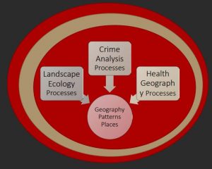
In the opening lecture of the course we were briefly introduced to the main topics that we would be reviewing for the remainder of the semester. These topics included: landscape ecology, health geography and crime analysis. We also went over the 5 ‘P’s in geography: patterns, places, processes, people and perspective.
Lecture 2 – Why is ‘geography’ important?
The fundamental issue:
“The problem of pattern and scale is the central problem in ecology, unifying population biology and ecosystems science, and marrying basic and applied ecology. Applied challenges… require the interfacing of phenomena that occur on very different scales of space, time, and ecological organization. Furthermore, there is no single natural scale at which ecological phenomena should be studied; systems generally show characteristic variability on a range of spatial, temporal, and organizational scales.” (Levin 1992; italics added)
In this lecture, the focus was that scale can be an issue for any type of spatial analysis and that within this, the scale is determined by the analyst. Other issues discussed were as follows: the modifiable areal unit problem (MAUP), the nature of the boundaries of a study area, and spatial dependence/heterogeneity. If you understand these issues you can work with the restrictions that they impose when working with spatial data. An important scale differentiation that was noted in this lecture was the difference between ‘grain’ and ‘extent’. Grain is the lowest resolution of the data, and extent is the scope or domain of the study area. MAUP is endemic to all spatially aggregated data. Gerrymandering is an example of how the MAUP can be taken optimized for political advantage (especially in the US). There are clear issues that need to be addressed when working with spatial data and understanding these issues shows how important geography can be.
Lecture 3 – Understanding landscape metrics: patterns and processes
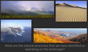
In this lecture the methodological considerations of spatial autocorrelation and stationarity along with processes, such as abiotic, biotic, anthropogenic and disturbances were discussed. Landscape structure (form) and quantification of pattern were also discussed. Spatial autocorrelation is a measure of the degree to which a set of spatial features and their associated data values tend to be clustered together in space (positive spatial autocorrelation) or dispersed (negative spatial autocorrelation) (from ArcGIS dictionary). A process is deemed ‘stationary’ if the processes that govern the placement of an object or event do not change over space/do not drift over space. Every geographic study has different processes at play. For example, to model urban sprawl numerous processes must be considered such as land use change, population growth rate, infrastructure development, etc. The number of processes for different geographic problems is endless! Important conclusion: “Remember, behind any analysis must be an understanding of the processes you feel are important on that landscape, an understanding of the scale at which those processes operate, and knowledge of how those processes impact the landscape.”
Lecture 4 – Statistics: A review
Understanding statistics is crucial when working with GIS as many outputs produce statistical outputs that are only useful if the analyst can interpret the meaning of the output statistics. For example, the Moran’s Index informs the analyst of the magnitude of spatial autocorrelation.
In this lecture, the focus for statistics was in regards to regression analysis. The Ordinary Least Squares (OLS) model was discussed as an example of regression analysis. The OLS is used to determine the relationship of dependent and independent variables. Regression is achieved by Geographically Weighted Regression (GWR), where the coefficients determine the weights for the regression.
Lecture 5 – What is Health Geography?
In this lecture, we explored the transition from “Medical Geography” to “Health Geography” through the idea of a post-medical geography of health. Five strands of Health Geography were discussed:
- Spatial patterning of disease and health
- Spatial patterning of service provision
- Humanistic approaches to ‘medical geography’
- Structuralist/ materialist / critical approaches to ‘medical geography’
- Cultural approaches to ‘medical geography’
“The discipline has traditionally been divided into two fairly distinct fields: one examines the geographical factors which contribute to ill-health and disease (geographical epidemiology); whereas the other deals with geographical factors influencing the provision of and access to health services (geography of health care).” – Klinkenberg, 2018
With any geographic topic the idea of “place versus space” needs to be understood. In Health Geography the emphasis is on places as opposed to space. This means that the focus is on the physical locations and their unique characteristics as opposed to relationships of points. The field of Health Geography is extensive. Some Health Geography research areas include:
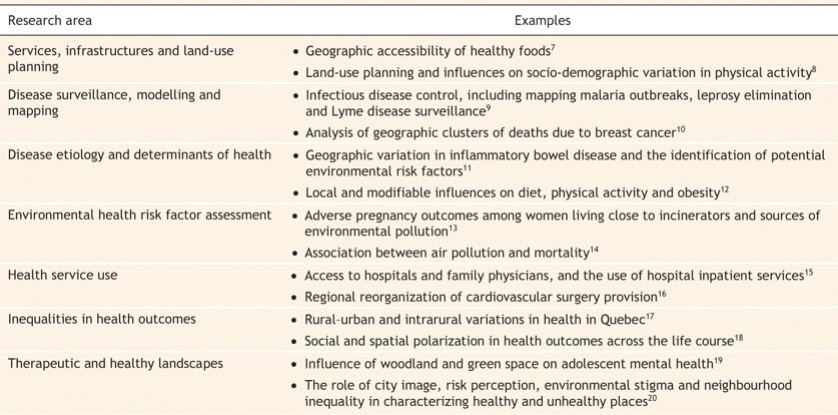
click image for higher resolution version (from Dr. Trevor Dummer’s report at this link: http://www.cmaj.ca/content/178/9/1177.full)
Lecture 6 – GIS in Health Geography
How can GIS be used in Health Geography?
“Health and ill-health are affected by a variety of lifestyle and environmental factors, including where people live. Characteristics of these locations (including socio-demographic and environmental exposure) offer a valuable source for epidemiological research studies on health and the environment. Health and ill-health always have a spatial dimension, therefore. More than a century ago, epidemiologists and other medical scientists began to explore the potential of maps for understanding the spatial dynamics of disease.” – Scholten and Lepper, 1991
There are four major applications of GIS in Health Geography:
- Spatial epidemiology
- Environmental hazards
- Modelling health services
- Identifying health inequalities
Spatial epidemiology is concerned with describing and understanding spatial variation in disease risk. As globalization has interconnected countries thousands of kilometres apart and air travel networks are so extensive, the risk of disease expansion is certainly a growing concern for countries’ domestic health security. Spatial epidemiology is a process that, through the assistance of GIS, can predict disease related risk such as the risk associated with globalization and flight networks. The next major application, environmental hazards, is the process for dealing with such things as water piping leakage. Modelling health services is critical to ensuring that all citizens have access to required healthcare. To add to this, identifying health inequalities can show regions where more health infrastructure investment is required.
Lecture 7 – Is crime related to geography?
GIS is also important in conducting crime related analyses. As the figure below shows, crime opportunity can be calculated by determining the likelihood of an offender presence, the presence of a suitable target and whether there is a capable guardian present.
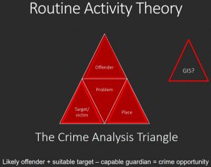
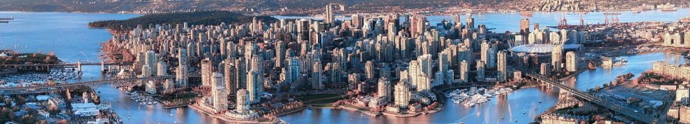
With this ideology in mind, there is a clear ability to apply GIS techniques in determining crime opportunity. For example, if we were to look into car thefts in Vancouver. We would have numerous data layers such as, known theft locations, overnight parking locations, police stations and possibly some demographic data such as income. With these data layers we could relate the three variables (offender likelihood, target suitability and guardian presence) in the equation for crime opportunity.
In this lecture we also discussed the Routine Activity Theory (RAT). “If we are to assume that routine activities affect the time of the criminal event, we only need to look at those activities to see that they are spatial. Residential and commercial areas are not randomly located, different areas have different magnitudes of renting/owning, age composition of the resident population, etc.” (Klinkenberg, 2018) Therefore, RAT, simplifies crime related issues to make GIS analysis more manageable. However, with simplification comes the issue of over simplification. So, when applying RAT in GIS analyses, this limitation should be understood. The figure below shows an example of routine activity that could be used in crime related GIS applications.

Click image for higher resolution version
Other theories such as Rational Choice Theory and Crime Pattern Theory were also discussed in this lecture and can understanding of these theories can also aid in GIS execution of crime related data. In summary, the three important environmental crime theories were summarised as follows: Routine Activity theory gives us a model to predict if a crime has all the right ingredients to occur, and Rational Choice Theory gives us some insight into what an offender is thinking when they decide to commit the crime, while Criminal Pattern Theory helps us understand where and when the offence will occur.
Lecture 8 – Use of GIS by Fire Departments
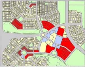
In this final lecture on applications of GIS, we explored how Fire Departments use GIS to better serve citizens and ensure that emergency situations can be dealt with most efficiently. This lecture focussed on Fire Departments in Calgary. Since Calgary is Canada’s “fastest growing city” (Bruce McBride from City of Calgary, 2005) there is ample opportunity and need for GIS use in order to ensure the safety of all Calgarians. By creating a risk map that follows the following definitions, city planning could ensure that everyone within the city boundaries was covered by rapid response Fire Department, and if they were not, this could be addressed.
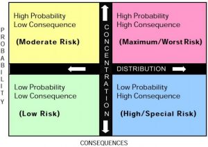
By using the above criteria, maps like the map shown could be developed with GIS in order to highlight high risk zones. This could aid in redevelopment and policy efforts.