In this course four lab reports were created. Click on the links below to see the lab instructions. Scroll down further to view brief summaries of each lab and links to my lab reports!
Lab 1 – Spatial stats using Modelbuilder
Lab 2 – Exploring Fragstats
Lab 3 – Introduction to Geographically Weighted Regression
Lab 4 – Introduction to CrimeStat
Summaries of each lab report
Lab 1 – Spatial stats using Modelbuilder
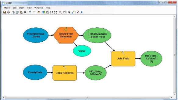
Modelbuilder – click on image to view higher resolution image
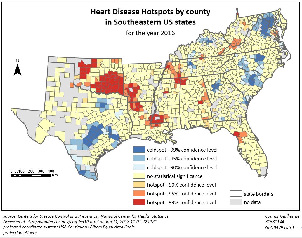
Final map – click on image to view higher resolution version
summary: In this brief lab, we learned how to use Modelbuilder. Modelbuilder is a very useful aspect of ArcGIS as it allows the analysis to develop a methodology for data analysis that can be altered slightly to determine a varying range of outputs. For example, for the course final project I was able to use Modelbuilder to run through numerous ‘weighted sums’ for range of outputs with different inputs and different weighting regimes. This ensured consistency and reduced analysis time. For this lab, Modelbuilder was used to create a hot spot map of Heart Disease in the US for 2016. Two models were created in order to 1) process the data into individual feature classes (for each year) and 2) to perform the hot spot analysis for each year’s feature class.
Click this link to view report: Lab 1 report
Lab 2 – Exploring Fragstats
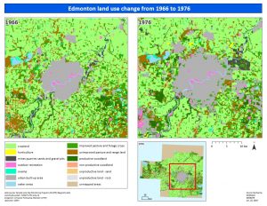
Final map – click on image to view higher resolution version
summary: In this lab, Fragstats was used to determine landuse change. In particular, urban sprawl and rural urbanisation were analyzed and the most affected land use type from 1966 to 1976 was determined for the City of Edmonton. Fragstats software was used to Fragstats to identify class level and landscape level metrics in order to help determine the change from 1966 to 1976. By comparing the land use data attained by the Canada Land Use Monitoring (CLUMP) data from 1966 and 1976, this analysis showed that there was a decrease in the number of patches of the following land use types: unimproved pasture and range land (-879 patches), improved pasture and forage crops (-417 patches), productive woodland (-440 patches) and swamp, marsh or bog (-593 patches). The total core area increased more for the urban built up areas land use type than any other land use type. From 1966 to 1976, the total core area for urban built up areas increased from 15,708ha to 38,268ha and the core area percent of landscape increased from 2.43% to 5.94%.
Click this link to view report: Lab 2 report
Lab 3 – Introduction to Geographically Weighted Regression
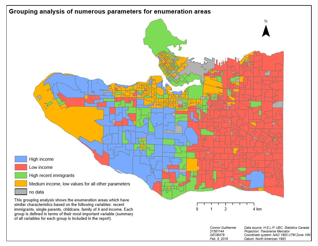
Output map – click on image to view higher resolution version
summary: In this lab, we were introduced to working through a Geographically Weighted Regression (GWR) to determine the factors that most influence “social skill” in Vancouver. The GWR is a powerful tool in understanding and quantifying the relationships between a subject of interest and explanatory variables through both determining statistical and geographical significance. However, as the GWR is based on linear regression the model produced can only represent linear relationships even when in reality the relationship between variables maybe non-linear. The first step in regression is to run an Ordinary Least Squares (OLS) regression for the important explanatory variables (excluding any unimportant variables). In order to determine the “important” explanatory variables, the explanatory regression tool should be used prior to conducting the OLS. This tool determines the AdjR2 and the AICc for each variable – the most important variables have the highest AdjR2 values and the lowest AICc values. The OLS provides a model for the dependent variable and creates a single regression equation to explain the dependent variable. It is important to run the GWR with the same input variables as the OLS as this will ensure that consistency in the relationships the model identifies. Based on the GWR conducted for Vancouver it appeared that there was a relationship between low income areas and social skills. It also showed that language ability/score plays a significant role in determining social skill.
Click this link to view report: Lab 3 report
Lab 4 – Introduction to CrimeStat

Output map – click on image to view higher resolution version
summary: For the final lab report for this course, CrimeStat was used in conjunction with Moran’s I, fuzzy hot spot analysis, nearest neighbour hierarchical spatial clustering, Knox index and kernel density to analyze break and enter and car theft data in the City of Ottawa. Through the use of the nearest neighbour index and Moran’s index, spatial autocorrelation of crime in the city was determined. Hot spot analysis and nearest neighbour hierarchical spatial clustering techniques were used to map residential break and enter crimes. Both non-risk adjusted and risk-adjusted clusters were determined for the residential break and enter crime data to determine the influence of including population in the cluster calculation. The Knox index was used to test the spatial and temporal clustering of car theft based on the location of the crimes and the time of day that they occurred. Finally, single and dual kernel density maps were created to show the interpolated residential break and enter crime intensity for the entire study area. Through these analyses techniques, this report shows that there is significant influence of environmental factors, such as land use and population, on crime in the city of Ottawa.
Click this link to view report: Lab 4 report