
Air pollution is a mix of hazardous substances, and can have both anthropogenic and natural sources. Anthropogenic sources include emissions from vehicles, industry, power generation, and chemical production (NIH). Natural sources include forest fires and volcanic eruptions. Air pollution is a public health issue, correlating to many diseases. Most directly, this includes respiratory and lung diseases, including asthma, emphysema (shortness of breath), bronchitis, and chronic obstructive pulmonary disease (NIH). More alarmingly, recent science has shown that air pollution can impair blood vessel function, resulting in cardiovascular diseases such as heart attack and stroke. With prolonged time frames, air pollution has been shown to correlate with cancer (NIH).
The estimates of the impact air pollution has on our health is staggering. Over 90 percent of Californians breathe unhealthy levels of one or more air pollutants during some part of the year (CARB). This parallels the global estimate, with 9 in 10 people breathing in polluted air (WHO). In addition, according to the America’s Health Rankings Annual Report of 2021, California has the worst air pollution out of any US state. Globally, the WHO estimates that every year, air pollution is blamed for the deaths of 7 million people, and one-third of deaths from stroke, lung cancer, and heart disease.
Air pollution is hard to escape because air circulates across space and over time. Many studies have investigated the spatial and temporal dynamics of air pollution. However, air pollution is not random. It disproportionately impacts those living near pollution sources such as highways and factories. Often these are poor, racialized, and other marginalized communities. In California, CalEnviroScreen was developed to help identify California communities that are disproportionately burdened by multiple sources of pollution, and where people are often vulnerable to the effects of pollution. It was developed by CalEPA and the Office of Environmental Health Hazard Assessment (OEHHA). It analyzes data on environmental, public health and socioeconomic conditions in California’s census tracts to produce scores of cumulative pollution burdens and vulnerabilities throughout the state.
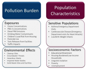
Although CalEnviroScreen was designed to assess cumulative pollution burdens, the variables processed with reliable data sources by experts in GIS and public health presents a wealth of data for a GIS analysis. The variables are categorized into pollution burden and population characteristics.
Research Objectives
Our novel analysis focuses on the exposure variables related to air pollution and how they correlate to sensitive populations in two cities in California, using a selection of variables from CalEnviroScreen.
The explanatory variables representing air pollution exposure include ozone, PM2.5 (fine particulate matter), Diesel PM, Toxic Releases from Facilities, and traffic impacts. The dependent variables representing sensitive populations include asthma and cardiovascular disease, which are known throughout the scientific community to be correlated to air pollution. Air pollution is one of the main contributors to cardiovascular and respiratory diseases worldwide (Requia et al, 2016).
Ground-level ozone is the primary component of smog (CalEnviroScreen Report).
PM2.5 is defined as particles that have a diameter of 2.5 micrometers or less. It is a complex mixture of aerosolized solid and liquid particles including such substances as organic chemicals, dust, allergens, and metals. These particles can come from many sources, including vehicles and industrial processes (CalEnviroScreen Report).
Diesel PM is the particle phase of exhaust emitted from diesel engines commonly used to power trucks, buses, cars, trains, and heavy-duty equipment. Also known as soot, Diesel PM is composed of a mixture of compounds, including sulfates, nitrates,
metals and carbon particles (CalEnviroScreen Report).
Toxic releases are defined as emissions from facilities, including factories, into the air (CalEnviroScreen Report).
Traffic is a significant source of air pollution in most urban areas across the world (Requia, 2017). It is defined as vehicles on the road (CalEnviroScreen Report).
Asthma is a chronic lung disease characterized by episodic breathlessness, wheezing, coughing, and chest tightness (CalEnviroScreen Report). Asthma increases an individual’s sensitivity to pollutants. Asthma rates are a good indicator of population sensitivity to environmental stressors because asthma has been found to both be caused by and worsened by pollutants (Guarnieri & Balmes, 2014).
Cardiovascular disease (CVD) refers to conditions that involve blocked or narrowed blood vessels that can lead to a heart attack or other heart problems. Individuals who have had a heart attack may have a higher risk of dying after exposure to both short- and long-term increases in air pollution (CalEnviroScreen Report).
Study Area
In terms of the study area, we selected the two largest cities in California, Los Angeles, and San Francisco, and their respective metropolitan areas. The Los Angeles Metropolitan Region consists of LA County and Orange County, and includes the cities of Los Angeles, Anaheim, and Long Beach (Figure 1). It has a population of 13,211,027 and an area of 4,852.1 square miles (https://censusreporter.org/profiles/31000US31080-los-angeles-long-beach-anaheim-ca-metro-area/). The San Francisco Bay Area consists of 9 counties: Alameda, Contra Costa, Marin, Napa, San Francisco, San Mateo, Santa Clara, Solano, and Sonoma (http://www.bayareacensus.ca.gov/counties/counties.htm & Figure 2).
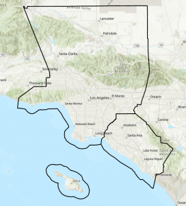
Figure 1. Metro LA counties and boundaries
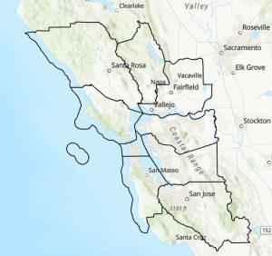
Figure 2. San Francisco Bay Area counties and boundaries
Research Questions:
- How does the relative ratio of the different air pollutants differ between communities?
- Which communities have the highest air pollution burden of the combined 5 air pollutants?
- Which air pollutants have the highest correlation with asthma and cardiovascular disease in each city?
- Which regression model is the best fit?
- What are the differences between the two cities?