In this lab, we used multiple methods to demonstrate how various crime incidents can be spatially distributed and visualized. We were introduced to CrimeSTAT, which is a spatial statistics program for the analysis of crime incident locations. Our study area was Ottawa, Ontario between January 2005 and March 2006. The crimes analyzed were residential and commercial break and enters (B&E’s) and car theft. This lab highlighted that by adjusting statistics for baseline population differences, you can end up creating a significant difference in the interpretation results.
The following are the different methods to analyze data used in CrimeStat.
Nearest Neighbour Index
According to Levine (2010), the nearest neighbour index is a test of “whether the average nearest neighbour distance is significantly different than would be expected on the basis of chance” (p. 6.6). The nearest neighbour analysis determines the pattern of activities and shows evidence of clustering of crime or whether it is dispersed. Analysis is based on the points themselves. An index value close to 1 means total spatial randomness and a value closer to 0 indicates strong spatial clustering. We can observe (Figure 1.) that overall, the first order recorded crimes in Ottawa are more spatially aggregated than expected. We can also observe (Figure 1.) how the nearest neighbour index changes as a function of the type of crime, where commercial break and enters have the lowest nearest neighbour index and residential break and enters have the highest index. Commercial break and enters have the strongest spatially aggregated neighbours most likely due to zoning laws and the fact that commercial businesses are generally closer together than residences or cars.
All of the nearest neighbour indexes increase as the nearest neighbour order increases. This demonstrates that the clustering of crime incidents are only significant up until about the 4th order of nearest neighbours. As you include more neighbours in analysis, the distribution of crime becomes more dispersed.
Moran’s Correllogram
While the nearest neighbour index looks at the individual points themselves, Moran’s I considers the aggregation of points within an enumeration unit, so Moran’s Correllogrram looks at the intensity of points within the dissemination areas (DA) of Ottawa. The zones, or the DAs, become the unit of analysis instead of the individual data points. This can garner different results because “zones have attributes which are properties of the zone, not of the individual event” (p.5.4 Levine 2010).
When comparing the nearest neighbour results (Figure 1) to Moran’s corellogram results (Figure 2), we can observe two different stories. Moran’s values closer to 1 indicate a stronger spatial autocorrelation and values closer to 0 depict more diffusion, opposite values used by the nearest neighbour index. The Moran’s corellogram results depict that residential break and enters have the strongest spatial autocorrelation. This is providing information about the scale of autocorrelation and depicting “the extent to which ‘hot spots’ are truly isolated concentrations of incidents” (p. 5.30 Levine 2010). The Moran values differ between residential B&E’s and population because the highest population densities generally occur in one general area, the downtown core, enforcing almost a limit to how spatially correlated it can be. Whereas residential B&E’s can reveal a stronger spatial autocorrelation because this land use is more spread out increasing the potential for clustering.
Fuzzy Mode vs Nearest Neighbour Hierarchical Spatial Clustering
The fuzzy mode clusters observed (Map 1.) are visualizing crime events that occur around or near a location. They are defined by a 500m radius around each point to include events that occur around or near that location. This analysis depicts hot spots as locations with the most number of incidents (Levine 2010).
The nearest neighbour hierarchical spatial clustering results “are like an inverted tree diagram in which two or more incidents are first grouped on the basis of some criteria. Then pairs are grouped into second-order clusters” (p. 7.2 Levine 2010) and so on. The difference between the fuzzy mode and the hierarchical spatial clustering is that the latter clusters the volume of incidents whereas the former merely indicates areas with high volumes of crime in relation to its specified neighbours (in this case 25).
Nearest Neighbour Hierarchical spatial clustering vs Risk-adjusted Hierarchical spatial clustering
The main difference between the standard nearest neighbour hierarchical spatial clustering results and the risk-adjusted results is the standard routine identifies areas with a high volume of crime and the risk-adjusted routine identifies areas of high risk for crime, “it is a risk measure, rather than a volume measure” (p.7.11 Levine 2010). So in the NNH routine, it clusters points without taking into consideration of where they are occurring, “the threshold distance is constant throughout the study area” (p. 7.11 Levine 2010). But in the RNNH, it uses a baseline variable, in this case, population density, and adjusts the threshold distance according to what would be expected of that baseline variable.
The hierarchal clusters observed (Map 1.) are first, second, and third order risk-adjusted clusters. Basically, the first order clusters are clustering the individual crime incidents but normalized to population density. The second order clusters are clustering the first order clusters. This is useful to compare high risk areas in the city rather than just localized incidents, it “increases the ease of use for analysts and can facilitate comparisons between different areas without having to limit arbitrarily the data set” (p. 7.16 Levine 2010). The third order cluster in this data set is not depicting much due to the scale, as it encircles the majority of the study area.
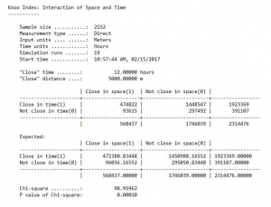
Knox Index
The Knox Index is a simple measure of space-time clustering (Levine 2010). This means that individual pairs of recorded car theft are compared in terms of distance and in terms of time intervals. Close in space for the Knox results in this dataset (Figure 3) is defined as pairs of car theft incidents that occur within 5km. Close in time represents pairs of incidents that occur within 12 hours.
After running 19 simulations in order to gage whether results would be random or not, the Knox Index results determined a Chi-square test larger than 98% meaning that the null hypothesis of a random distribution between space and time is rejected. Car thefts appear to be more clustered in space and time compared to the expected results (Figure 3).
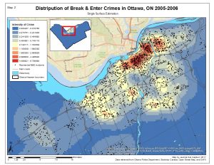
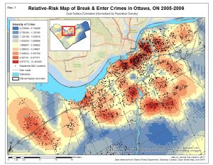
Kernel Density Estimation
The Kernel Density Estimations create a surface that generalizes crime incidents to an entire area basically interpolating density estimates. In contrast, spatial distribution hot spot statistics provide statistical summaries for the data incidents themselves (Levine 2010). The intensity variables (Map 2 & Map 3, intensity of crimes) is depicting areas of the city with the highest intensity of residential B&E’s.
The single surface estimation (Map 2) is similar to the fuzzy mode of clustering results because the surface is interpolating the volume of crime. The highest intensity of crime is occurring in the downtown core, not surprisingly due to the high density of population.
The dual-surface estimation is similar to the risk-adjusted clusters because it is using population as a secondary variable. Therefore, areas that are considered at a high risk for residential B&E’s represent higher crime intensities.
Appendix
Figure 1. Nearest Neighbour Index
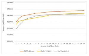
Figure 2. Moran’s Correlogram
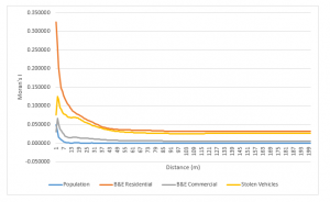
Figure 3. Know Index Results
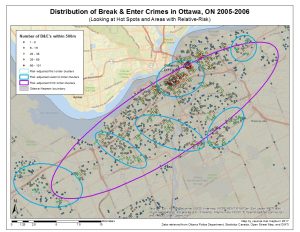
Map 1. click here to enlarge.
Map 2. click here to enlarge.
Map 3. click here to enlarge.
Reference
Levine, N. (2010). CrimeStat: A Spatial Statistics Program for the Analysis of Crime Incident Locations (v 3.3). Ned Levine & Associates, Houston, TX, and the National Institute of Justice, Washington, DC. July.