Monthly Archives: April 2019

The first lecture centers around the introduction of GIScience and its application in research. Specifically, it is applied in three major fields which the class will dive into intensely throughout the school term. The three fields are landscape ecology, crime analysis, and health geography. Though they seem different, but they share the core 5 P’s principle which are patterns and processes, places, people and perspectives.

Landscape Ecology: The study of how landscape structure affects the abundance and distribution of organisms. The goal of ecological research is to understand how the environment, including biotic and abiotic patterns and processes, affects the abundance and distribution of organisms.

Health Geography: Health geography is a subdiscipline of human geography, which deals with the interaction between people and the environment. Health geography views health from a holistic perspective encompassing society and space, and it conceptualizes the role of place, location and geography in health, well-being and disease.

Crime Analysis: Crime analysis is a systematic analysis for identifying and analyzing patterns and trends in crime and disorder. Information on patterns can help law enforcement agencies deploy resources in a more effective manner, and assist detectives in identifying and apprehending suspects. Crime analysis also plays a role in devising solutions to crime problems, and formulating crime prevention strategies.

In this lab exercise I took a look at the crime cases in the Ottawa area, specifically, break and enter in the commercial and residential areas as well as car thefts. Using the program CrimeStat, I was able to conduct several spatial distribution analysis such as nearest neighbour index, fuzzy hot spot analysis, knox index, and kernel density.

In the first analysis I used the nearest neighbour index. The purpose of this is to
analyze the distance between each crime and the 25 closest instances of the same crime. The nearest neighbor index is the ratio of the observed nearest neighbor distance to the mean random distance of the crime took place, therefore, the index compares the average distance from the closest neighbour to each point with a distance that would be expected on the basis of chance.

The hot spot and clustering analysis allows map reader to visualize where exactly
crimes are being committed in Ottawa. The first hot spot analysis used in this lab is the fuzzy mode analysis. These clusters are visually represented by coloured circles on the map below. The colours of the circle represented with a tool which quantifies the number of other crimes within 1000 metres radius. For instance, the red circles represent crime sites where 187 to 247 of crimes are within 1000 metres, orange circles represent crime sites where 136 to 186 of crimes are within 1000 metres, and green circles represent crime sites where 1-78 of crimes are within 1000 metres.

On the other hand, the other method is the nearest neighbour hierarchical clustering analysis. The method identifies hot spot areas instead of circles on the map, therefore, creating zones of blue polygons shown on the map. The polygons portray hot spot areas that contains at least 10 crimes located within a 1000 metre area. When comparing the two hot spot analysis methods, I can visually see similar results produced by the two. In this application, the fuzzy mode analysis is superior where it provides readers with more information about the criminal activity within the area since it is able to provide the intensity (number) of the crime sites.

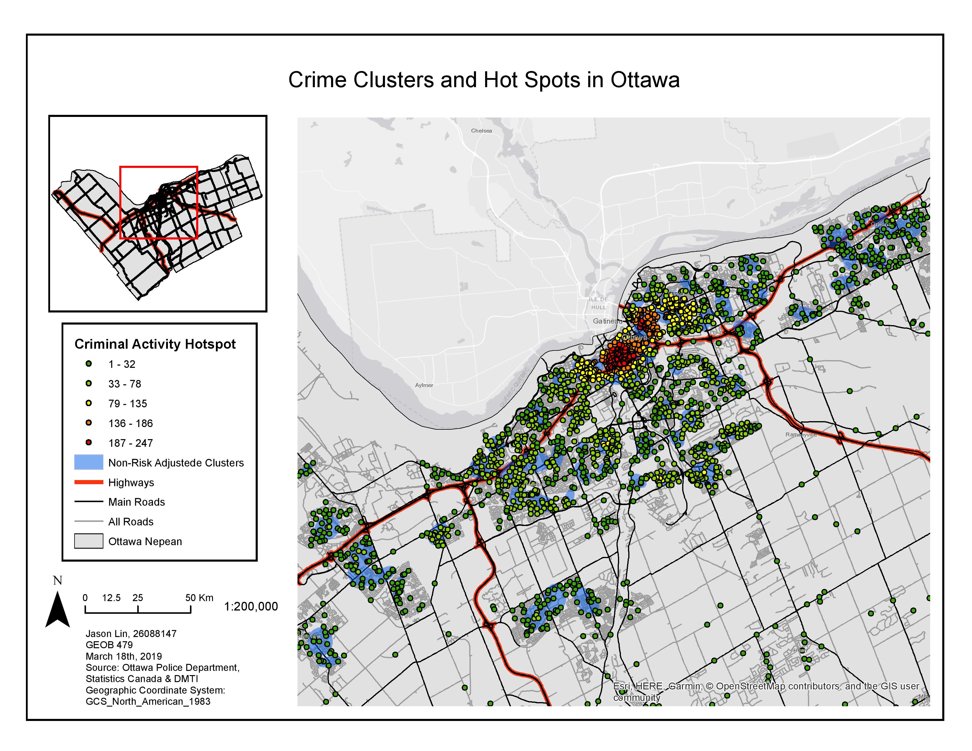
The nearest neighbour hierarchical spatial clustering method used previously was non-risk adjusted, meaning that the underlying conditions and factors to why these hotspots occurred is unaccounted for. Therefore, this could potentially be problematic because the relative risk to a person from crime within an area is affected by many elements such as population. When the risk adjustment is carry out, clusters of clusters are identified.

For my analysis on car theft I used the knox index, the knox index is used to determine whether there is a spatial and temporal clustering within a given data. I ran the analysis 19 times and I have defined the temporal element as close within 6 hours and distance element as close within 5000 metres. Specifically four numbers for each categories were produced: close in time and space (325473); not close in time and space (759110); and close in time and not close in space (986929); and not close in time and close in space (242964 ). Therefore, from the numbers, I can observe that car thefts tend to be close in time but not close in space, in another word, these crime happens depends on the time of the day rather than the location of the crime.

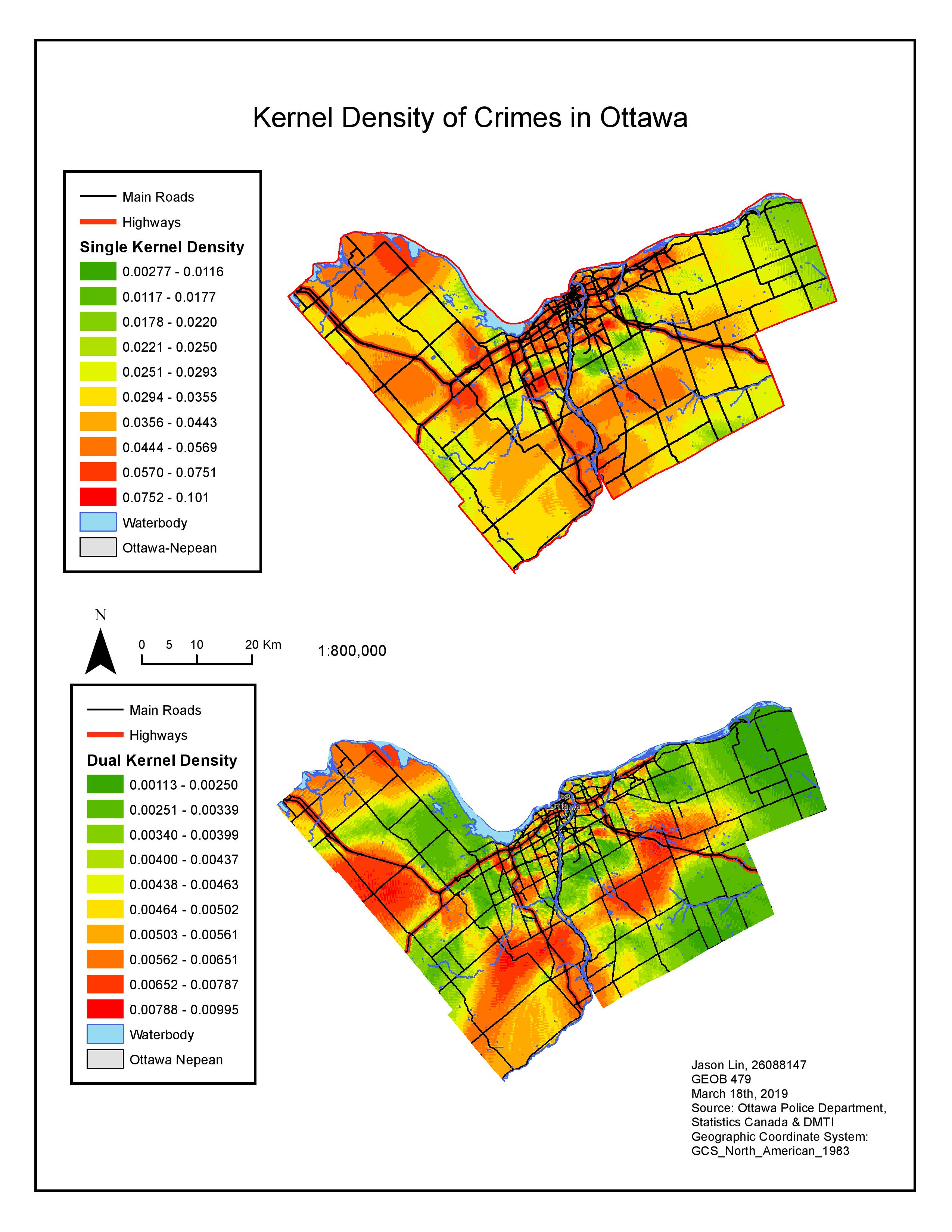
The last map shows the kernel density of the crime cases. Kernel density is a method where it interpolates crime data given to form a smooth surface showing the expected intensity of crimes over the study area. Contrasting with other hot spot analysis such as fuzzy mode and nearest neighbour clustering, kernel density method offers one major advantage, it offers the ability to visualize a broad, regional view of events.

In this lab exercise, I conducted an analysis using the geographically weighted regression to determine children’s language skills in relation to different set of variables such as family income, immigration, child care, and family composition, and all the variables will be influenced by the neighbourhoods in which they reside.

In ArcGIS, the geographically weighted regression model is a regression used to model spatial relationships of a given dataset. This regression model is useful in working with large data sets with multiple features, which we are working with multiple enumeration areas as our census data.

Additionally, I compared the statistical results of the geographically weighted regression and the ordinary leas square regression and see how they are reflected in one of my maps. Thus, I was able to make assumptions about why the regression models are better at predicating certain parts of Vancouver while lacking accuracy in other regions. Moreover, I discussed other uses of the GWR model by exploring the relationship between crime rate and lead exposure. The data used in the lab was collected by the Human Early Learning Partnership (HELP) at UBC, using the Early Development Instrument (EDI) questionnaire. Furthermore, census data was used in the grouping analysis, with spatial nits of the census data being in Enumeration Areas (EAs).

Another analysis I had conducted in order to address the regression model’s predicative capability was the grouping analysis shown by (Map 2). 4 Groups were created to address variables I had chosen which were childcare, family of 4, lone parenthood, recent immigrants, and income. From the result shown by (Map 2), I could identify two strong regions to discuss which are Vancouver East side (shaded in yellow), and areas around Kerrisdale (shaded in red). Their characteristics were shown by (Figure 1). Therefore, I could speculate that in the Kerrisdale region which has the highest income and lowest lone parenthood, the combination of these two variables may drastically reduce the importance of having strong language score, thus, reducing the predicative capability of the regression models

Map 1:

This map shows the predicative capability of the OLS and the GWR in explaining the influence of children’s language score on social skills.

Map 2:

This map shows the 4 groups that share similar characteristics of the social variables (recent immigrant, lone parenthood, childcare, family of four, and income).

In this first lab exercise, I explored the land use changes in Edmonton, Alberta from the year 1966 to 1967. Using the data gathered from the Canada Land Use Monitoring Program (CLUMP) from Geogratis website, our main objective is to examine the trend and changes in agricultural land and urbanization.

From the class metrics, I observed a significant decrease in agricultural land types as they are being converted into urban built-up areas. At the same time, I observed decreases from other agricultural land types: improved pasture and forage crops (2000 hectares), non-productive woodland (12,000 hectares), swamp marsh or bog (5000 hectares), unimproved pasture and range land (30,000 hectares).

Additionally, it may be helpful to understand which land use types are being converted into another using transition matrix. Transition matrix offers us a clear picture to examine these land use conversions. For example, looking at horticulture, I can see that in 1976, only 1.86% of the land was from 1966 originally, however around 85% of its new land were converted from cropland.

Overall, rapid land use changes took place between year 1966 to 1976, population growth has accelerated urbanization in Edmonton, Alberta. This can be seen clearly on both maps where they show both the zoomed in area of the city center and the suburban areas. Urbanization leads to several regional impacts such as fragmentation of different land use type and the reduction of agricultural land.

Transition Matrix showing changes in land use between different class types in Edmonton, Alberta between 1966 and 1976.