As discussed, landslides are complex phenomena occurring in various forms and requiring site-specific solutions. Their complexity is reflected in many of the GIS and computing methods that currently depict and estimate landslide susceptibility and hazards, which tend to be just as complex as landslides themselves often requiring advanced knowledge in fluid dynamics, coding, and in some cases software engineering. This greatly limits the accessibility of these tools to the general public. The goal of the tool discussed here is to be accessible and easily picked up by anyone wanting to understand landslide risk at a local scale. It is important to note that this tool is not a replacement for professional knowledge nor should it be used as an accurate replacement for a slope stability assessment conducted by a licensed engineer. The tool was designed to estimate slope stability based on a set of criteria for the public, educational and referential purposes. This project uses the tool to help guide design-based solutions to slope stability. It provides the opportunity for anyone, such as designers, to have a basic understanding of what affects slope stability and what areas are susceptible to failure, in this case, to help guide design-based solutions and have a preliminary understanding of landslide risk in a given area.
There are lots of variables that can affect the stability of a slope. Trying therefore to include all of them in an easy-to-use way would be unrealistic. There are, however, a few main factors that are easily modeled using GIS namely; slope, vegetation density, proximity to streams, and elevation as a proxy for rainfall.
Areas of higher slope are more likely to fail due to various reasons. Mainly it is due to the angle of internal friction of a given soil and due to the relative stress of gravity (Bobrowsky & Highland, 2013).
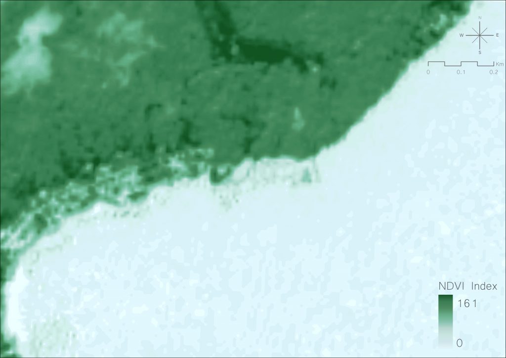
Vegetation density also affects slope stability as it stabilizes hills through root systems as well as through absorption of rainfall helping maintain a stable pore pressure within the soil. This can be calculated within ArcGIS Pro using the Normalized Difference Vegetation Index (NDVI), which uses spectral bands to evaluate vegetation density and health (Angers & Caron, 1998; Ford, 2016).
The elevation is used as a proxy for rainfall. It is well known that increased elevations often receive increased rainfall due to increased condensation through adiabatic cooling (Song, 2019; Smith, 2008).
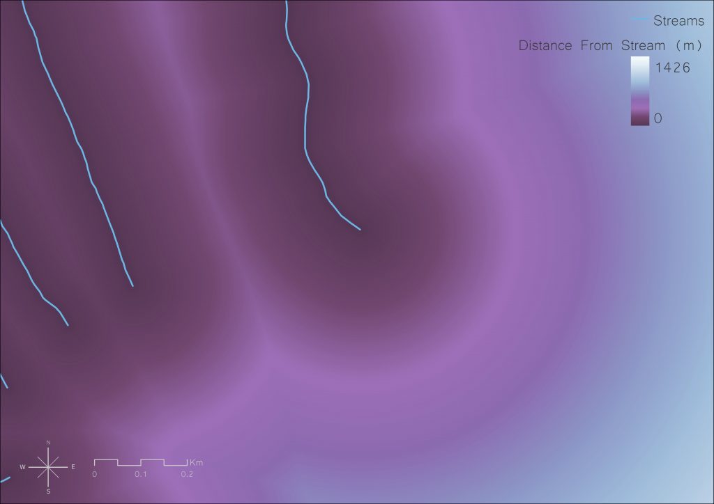
Proximity to streams was also important to include as streams greatly shape the landscapes they run through. Streams erode hillsides, increasing slope and in some cases undercutting them making them very likely to fail (Fox, 2010; Bobrowsky & Highland, 2013).
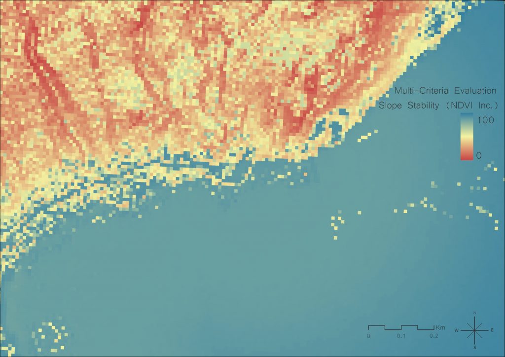
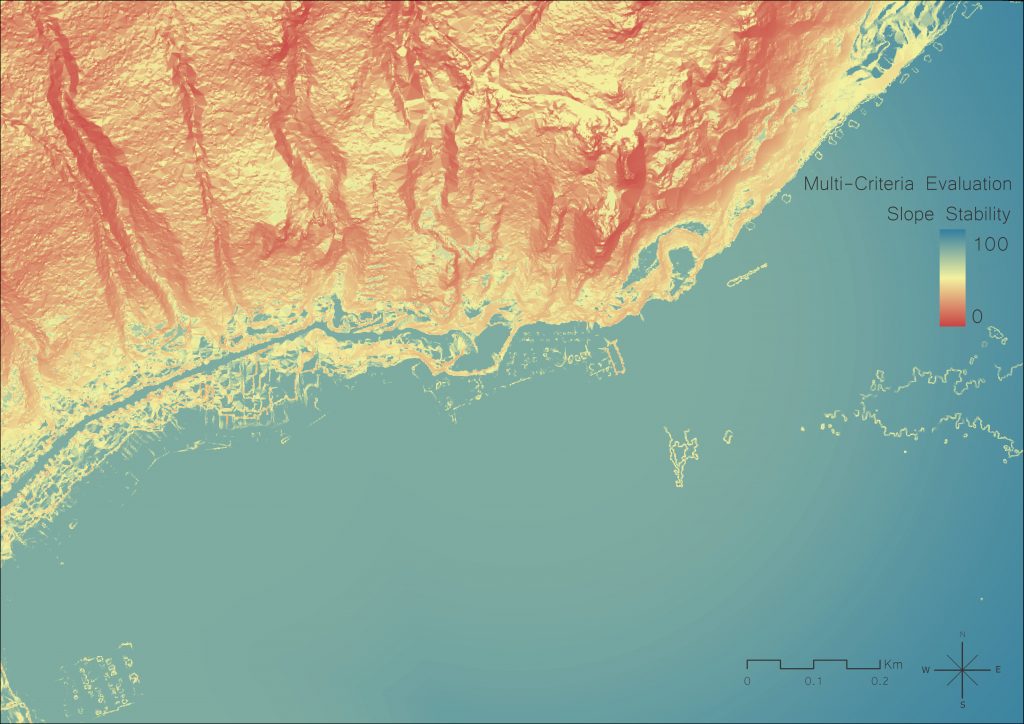
In order to evaluate slope stability, a Multi-Criteria Evaluation was conducted using the Suitability Modeler in ArcGIS Pro where each layer was assigned a weight which combined to a total of 100%. Within the layer itself, different values were assigned different weights using Transformation Functions in the suitability modeler. The result of this analysis is a slope stability map with values ranging from 1 to 100, where 100 is the most stable and 0 is the least stable based on the criteria imputed. Weights were assigned using the Analytical Hierarchy Process (AHP) that has been used by previous researchers to assign weights to different variables (Jazouli, 2019; Leonardi, 2020). AHP is a mathematical decision-making matrix that assigns weights based on the order of importance. In the case of landslide susceptibility mapping, this process is extremely useful as different variables should be assigned different weights based on the area of study (Cleveland, 2004).
This section outlines an example of a workflow to obtain the final suitability model using publicly obtainable data. As stated, the goal of this tool is to be accessible and usable by all and, while variable weight may vary by location, this tool can be applied to any location across the world as long as there is data present. Hopefully, anyone who chooses to follow the steps outlined below yields successful results.
Data & Software
Several different GIS software were considered when developing the tool. Finally, however, ArcGIS was the software chosen. This is because accessibility doesn’t only speak to a simple yet effective analysis, but also to the ease of use and price of software. Although ArcGIS isn’t free, it is without a doubt the most user-friendly of all GIS software with a minimal learning curve. The software may not be free however it is commonly available at libraries with public computers. Additionally ESRI, the software provider, offers a free trial period long enough to conduct several analyses.
The data used in this tool is summarized in the table below. The example study site was located in British Columbia, Canada and as a result, most of the data was publicly available through government databases. Multispectral satellite imagery used to calculate NDVI was downloaded through ESA’s Copernicus Open Data HUB. Although this type of satellite imagery is not of the highest resolution, it is the easiest to access and is adequate enough for this level of analysis.
| Data | Source | Format | Date |
| Level-2 Sentinel 2 Multispectral Satellite Imagery | Copernicus Access Open Hub | Raster – .tiff | 2022 |
| Study Area LiDAR | LiDAR BC | .laz | 2017 |
| Fresh Atlas Stream Network | BC Data Catalogue | Vector – .shp | 2011 |
Analysis
*preliminary note that the maps shown here are not the immediate output, colours and symbology has been changed but demonstrate the information. Instructions on how to change symbology can be found on ESRI.
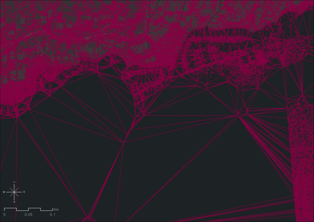
Processing LiDAR data in Arcgis
Open ArcGIS and navigate to the search bar at the top right, hover over it and a drop down menu will appear. Select Tools. Once the Tool pane opens, search for and open the “Convert LAS” tool. For the input LAS click on the folder and find your LAZ file. Next select the output folder. At the bottom select where you would like the out LAS file to be saved and name it. Leave all other options unchanged.
*If you cannot see your LAS file right click on it in the Contents pane on the left and select “Zoom to make visible”.
If your download LiDAR data was already in LAS format skip this step.
Right click on the LAS file under the contents pane and navigate down to LAS filters. A secondary menu will appear and select ground return. The map will update to the elevation of the ground only. This is important to do as the following layer will be created based on which filter is applied to the LiDAR file.
Next, in the tool pane, search for the “LAS to Raster” tool.
Select your LAS file as Input LAS Dataset. Below select the output location and name of the file to be created. At the bottom change the Sampling Value to “.75” Leave all other options as is. An example is shown below.
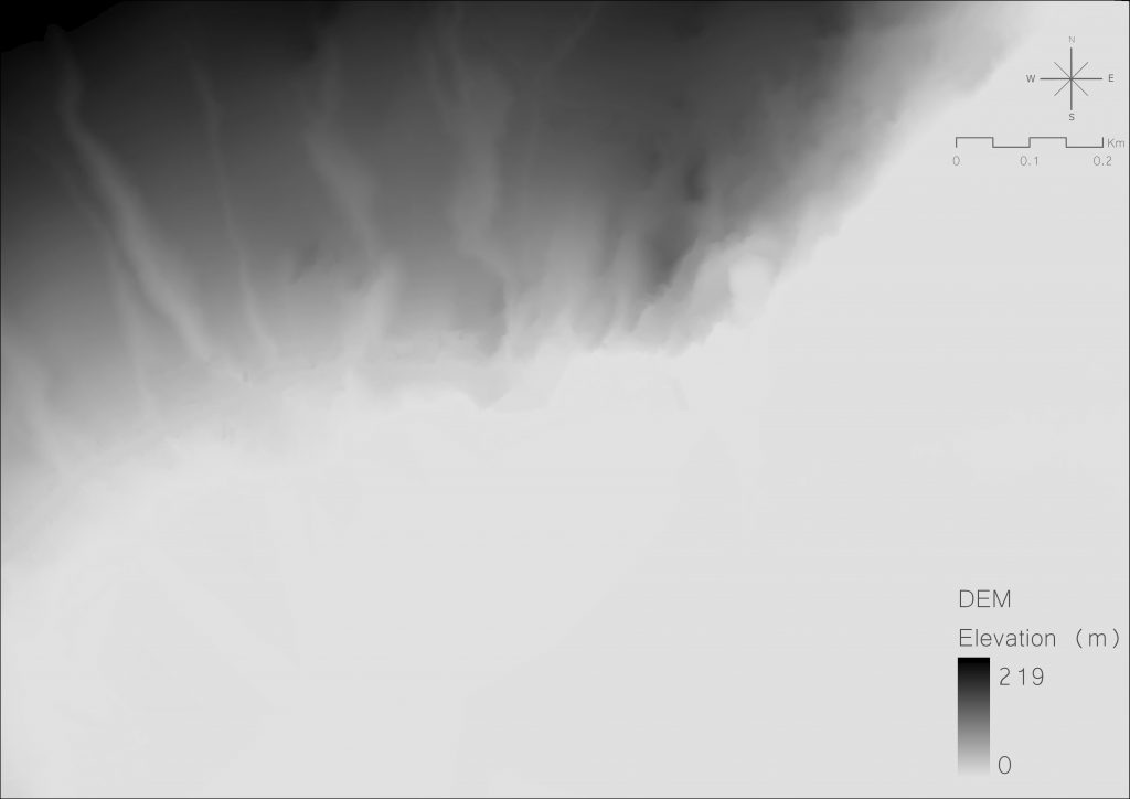
Once the tool is done running a Digital Elevation Model will be added to your map.
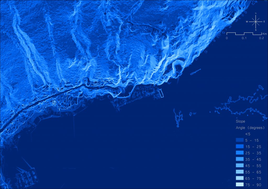
Navigate over to the tools pane again and search “Slope”. This tool creates a raster showing slope from your DEM. Open the tool and select your new DEM as the Input Raster. Select the output folder and name and leave all other options unchanged. Run the tool and a raster showing slope will be added to the map.
You now have your elevation layer as a proxy for rainfall and your slope layer.
Processing Stream Data & Calculating Distances from Streams
Next navigate to the map tab at the top of the window. Then select “Add data”. Search for your Streams Shapefile and add it to the map.
*When downloading stream data be sure to obtain as specific an area as possible to reduce computing times.
Next navigate over to the tools pane and search for “Euclidean Distance”. This tool will calculate the distance from the streams as an output raster file. For the input file or feature select the streams shapefile. Next, just below, name your output file and location. Leave the rest of the options unchanged and run the model. An output raster showing the distance to each stream should be created.
*If the output has a large cell size go back to the tool and change the output cell size until desired size is obtained.
You now have your distance from streams raster file.
Processing Multispectral Satellite Imagery and Calculating NDVI
Follow the steps above for adding the Satellite imagery to the map by navigating to the maps tab and selecting add data.
Once loaded a larger area of satellite imagery should appear on the map. This large tile increases computing time so it should be clipped.
Navigate to the tools pane and search “Clip Raster”. Open the tool and select the satellite imagery and the Input Raster. Select the file it will be clipped to, this can be any of the previous files such as the DEM. Once selected extent values will be automatically added to the 4 boxes below. Next select your output name and location and run the tool. A new layer will be created showing the satellite imagery that covers the same area as your other files.
Next is calculating NDVI. Navigate to the top of the window and click on the “Analysis” tab. Once open on the far right click on the “Raster Functions” button. A new pane will appear with several options. Click on NDVI. Select your clipped Satellite imagery as the input. Below you will have to select the red and near-infrared bands of your satellite imagery. If obtained from the Copernicus Open Data HUB red will be band 3 and near-infrared will be band 4.
If satellite imagery was obtained elsewhere search for band numbers in the images metadata or on the website where imagery was obtained. Click create new layer and an NDVI raster will be created.
Conducting a Multi-Criteria Evaluation to Determine Slope Stability
All four necessary files have now been obtained and the multi-criteria evaluation can be done.
Navigate to the Analysis tab once again and click the suitability modeler button. A new pane will appear. Click on the settings button in the pane and name your model. Then set the suitability scale to “1 to 100”. Right below change the “weight by” from multiplier to percentage. Lastly select the output raster name and location.
Click on the Suitability button next. In the box click the plus button and the finder window will appear. Find your four layers created and add them one by one. They are the Elevation raster, the slope raster, the NDVI raster and the distance from streams raster. Once all four are loaded click on the circle next to the Elevation raster in the box. It should turn green and a transformation pane will appear at the bottom of the window. In the Transformation window click Continuous function and click on the functions drop down menu and select MSSmall. This means that low values are more suitable (AKA receive less rain and are less likely to fail). Next click on the circle for the slope raster and a transformation pane will open for the slope raster. Once again navigate to continuous function and in the functions dropdown select small. This means slopes with a small number (low slope) are more suitable and less likely to fail. Do the same for the Distance from stream raster selecting MSSmall from the functions drop down menu. Lastly click on the circle next to the NDVI raster. Navigate to the continuous function once again. Click on the functions dropdown menu but this time select MSLarge. This is because a high NDVI value indicates denser and healthier vegetation which increases slope stability.
*more information of functions can be found here: The transformation functions available for Rescale by Function—ArcGIS Pro | Documentation
Before running the tool we have to assign weights. In the Suitability pane in the table showing our files on the right one can see the weights. In order to assign weights however one must use an AHP calculator to find the appropriate weights. Navigate to this website “AHP calculator – AHP-OS (bpmsg.com)”. Select 4 inputs and click OK. Follow the steps on the website. Remember that the values are variable based on locations but generally slope should have the most weight.
*There are several factors which affect slope stability and while many more layers could be added the goal was to keep this tool simple yet accurate. Depending on location priority of weights will vary based on importance of variables. AHP has been used by several studies and is an accepted scientific process. This text refers to Leonardi et al.’s analysis which was also conducted using AHP as a starting ground for assigning weights.
Once the weights are calculated go back to ArcGIS and fill the weights accordingly. Once they have been filled in, click “Run” at the bottom.
A suitability map should appear. The scale may not be from 0-100 as it is likely that there isn’t a single place that is 100% or 0% suitable. In these examples the higher values (higher suitability) are those less likely to fail. The lower value are less suitable (lower value) and are more likely to fail. The map that will appear will have a course resolution (large cell size). This is because of the NDVI layer which due to the satellite imagery has low resolution. If you wish to obtain a higher resolution imager simply exclude the NDVI layer from the suitability modeler and recalculate the weights.
Once the model is created you can right click on the layer in the contents pane, navigate down to symbology and change the colour scheme and more. You can also navigate to the insert tab at the top of the window and click on insert and then on layout to create a new layout where one can add legends, scales, titles and more.
Once again these results should just be used for educational referential purposes, they are not a substitute for professional analysis of slopes.
Limitations and Areas of Further Research
This tool, while effective and simple, has shortcomings that are noteworthy. While the tool provides a great and simple method for people to understand slope stability at a local scale and is applicable not only in several fields but around the world, its accuracy is limited due to the exclusion of certain variables. While the model prioritizes what are generally considered to be the most important factors in slope stability such as slope it generalizes by using elevation as a proxy for rainfall. It also excludes factors such as geology and land use which are important. The exclusion of these variable only modifies the output so much and would be included if data was available. The tool could be easily modified to include these layer by adding them into the AHP and Suitability Modeler, but in British Columbia the resolution of rainfall data and geology data is in the area of 1km per cell. That is to say an area of 1km by 1km is all classified as the same. The scale at which this analysis is conducted can therefore not include the data. This creates shortcoming in the model but also provides areas of future improvement and data sets become higher resolution and will be able to be added.
Another major limitation of this tool is that it does not calculate or model landslide runout. While this was initially a goal of this project there is currently no easy and accessible way to model landslide runout. This is because runout modelling require several inputs and a complex algorithm. Layers such as volume, water content, grain size and more are required to model runout. At the moment programs available for modelling run out require extensive knowledge in physics and computation. This is an area that requires extensive research are run outs zones are the areas where the majority of damage is caused. Developing an accessible way to model runout even if just for referential reasons is essential.
Bibliography
Angers, D. A., & Caron, J. (1998). Plant-induced changes in soil structure: processes and feedbacks. Biogeochemistry, 42(1), 55-72.
Bobrowsky, P., & Highland, L. (2013). The Landslide Handbook-A Guide to Understanding Landslides: A landmark publication for landslide education and preparedness. In Landslides: Global Risk Preparedness (pp. 75-84). Springer, Berlin, Heidelberg.
Cleveland, C. J., Gale Group, & Elsevier All Access Books. (2004). Encyclopedia of energy. Elsevier.\
El Jazouli, A., Barakat, A., & Khellouk, R. (2019). GIS-multicriteria evaluation using AHP for landslide susceptibility mapping in Oum Er Rbia high basin (Morocco). Geoenvironmental Disasters, 6(1), 1-12.
Ford, H., Garbutt, A., Ladd, C., Malarkey, J., & Skov, M. W. (2016). Soil stabilization linked to plant diversity and environmental context in coastal wetlands. Journal of vegetation science : official organ of the International Association for Vegetation Science, 27(2), 259–268.
Fox, G. A., & Wilson, G. V. (2010). The role of subsurface flow in hillslope and stream bank erosion: a review. Soil Science Society of America Journal, 74(3), 717-733.
Leonardi, G., Palamara, R., Manti, F., & Tufano, A. (2022). GIS-Multicriteria Analysis Using AHP to Evaluate the Landslide Risk in Road Lifelines. Applied Sciences, 12(9), 4707.
Smith, C. D. (2008). The relationship between monthly precipitation and elevation in the Alberta foothills during the foothills orographic precipitation experiment. In Cold Region Atmospheric and Hydrologic Studies. The Mackenzie GEWEX Experience (pp. 167-185). Springer, Berlin, Heidelberg.
Song, L., Chen, M., Gao, F., Cheng, C., Chen, M., Yang, L., & Wang, Y. (2019). Elevation influence on rainfall and a parameterization algorithm in the Beijing area. Journal of Meteorological Research, 33(6), 1143-1156.