Results
Based on the results from the Hotspot Analysis (Figure 1), there is a high concentration of crimes around downtown and a lower concentration of crimes as we move south. For statistically significant positive z-scores, the larger the z-score is, the more intense the clustering of high values (hot spot) (ESRI 2022). For statistically significant negative z-scores, the smaller the z-score is, the more intense the clustering of low values (cold spot) (ESRI 2022). Based on the z-scores, southern areas such as Shaughnessy, South Granville, and Dunbar-Southlands have seen increases in crime rates from 2006 to 2010 since their z-scores have gotten bigger. Despite still being relatively cold spots compared to the rest of the city, it would be interesting to see what socioeconomic changes in those areas contributed to the increase in crime rates.

Figure 1: HotSpot Analysis of 2006 and 2016 crime rates in Vancouver, BC
In Figure 2, there is a map highlighting the percent change in crime rates for each local area. Figure 2 is the difference between the two maps in Figure 1. Based on the results, it is easy to see that, the entire city of Vancouver has seen drastic reductions in crime rates from 2006 to 2016. However, interestingly, Shaughnessy was the only area to see a significant increase in crime rates, increasing by nearly 27%.
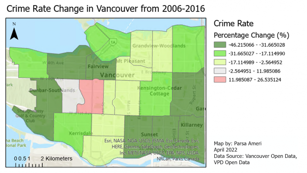
Figure 2: Crime rate change from 2006 to 2016 in Vancouver, BC
The results from our GLR help produce Figure 3 where the relationships between the change in each variable are shown. In terms of direct relationships, the change in crime rates and change in percent of the young population had an R2 value of 0.28 which was the largest value associated with crime rates. Besides that, other relationships found included an R2 value of 0.6 and 0.46 between the inverse of change in population density and change in lack of higher education and between the changes in low-income rate and change in percentage of lone-parent households, respectively.
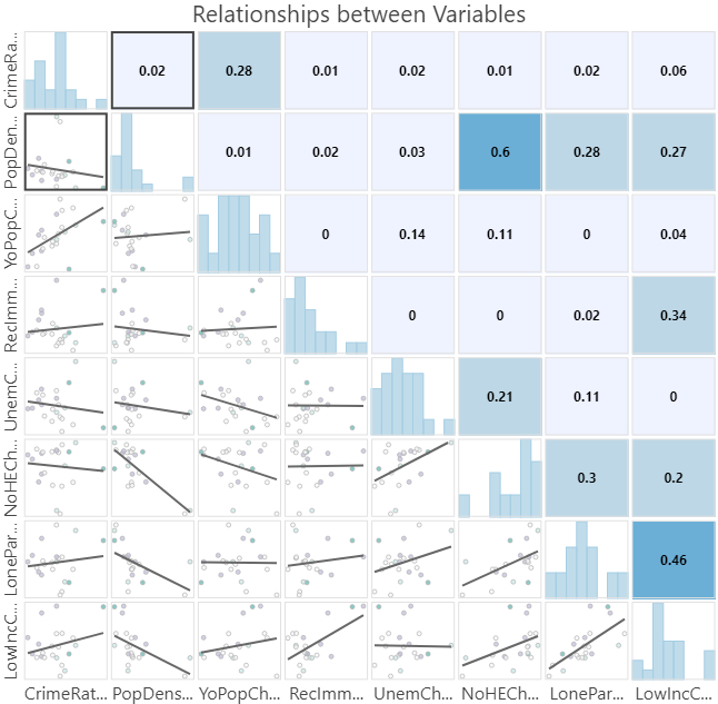
Figure 3: GLR results indicating relationships between all variables
Exploratory Regression Results
The Exploratory Regression produced five tables (Table 1,2,3,4,5), adding an additional variable every time to find the best combination of variables to explain crime rate change. Each table presents the three highest adjusted R2 values models.
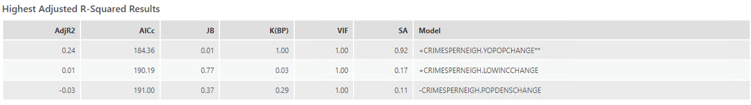
Table 1: Explanatory Regression results indicating the highest adjusted R^2 values for 1 variable
Table 1 shows the results for the strongest relationships between a single dependent variable and our independent variable, the change in crime rates. Unfortunately, only one of the three presented models shows any correlation at all with an R2 value of 0.24 for change in young population percentage, therefore agreeing with the results from Figure 3.
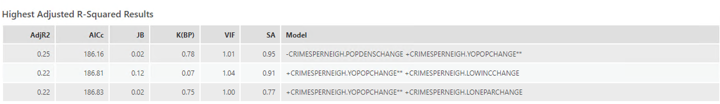
Table 2: Explanatory Regression results indicating the highest adjusted R^2 values for any 2 variables
In table 2, the highest adjusted R2 for any two variables is considered. The results are promising as we have some relatively high values compared to all other models. The change in young population percentage in combination with the inverse of the change in population density produced the highest R2 value of 0.25 meaning the combination of these two variables explains around 25% of the variation in change in crime rates. Following that, the combination of change in young population percentage with change in low-income households and change in lone-parent households both produced an R2 of 0.22.
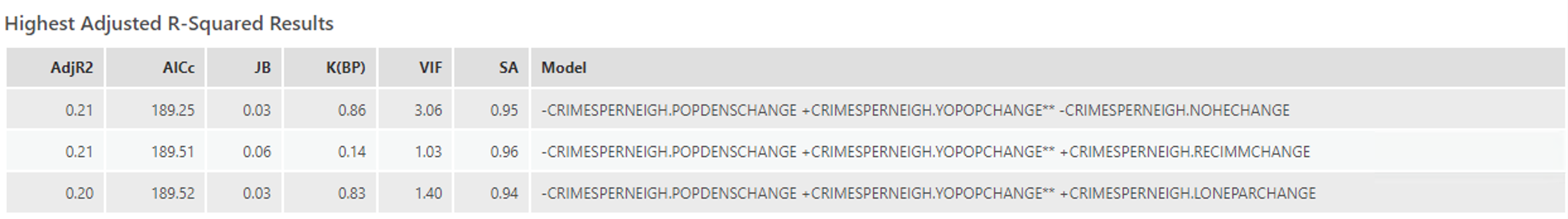
Table 3: Explanatory Regression results indicating the highest adjusted R^2 values for any 3 variables
When the combination of any three variables was considered, all three models presented include the inverse of change in population density with change in young population percentage (Table 3). The highest adjusted R2 value was when the change in lone-parent households’ percentage was added with a value of 0.21. Closely following that was when the change in no higher education percentage and change in low-income rate were added, both producing an R2 of 0.20.
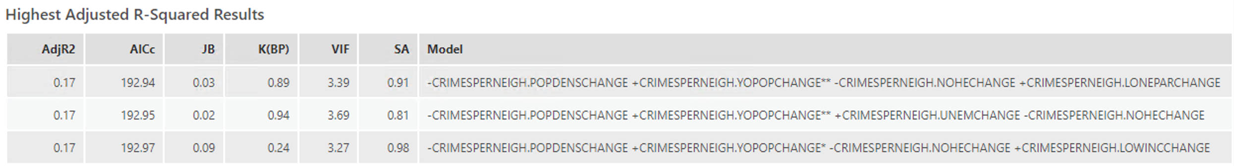
Table 4: Explanatory Regression results indicating the highest adjusted R^2 values for any 4 variables
Based on the combination of any four variables, none of our adjusted R2 were higher than 0.25 (Table 2). As we start to add more variables, there is less of a correlation between the change in socioeconomic variables and the change in crime rates. Notably, three socioeconomic variables were in all three models. These variables were the inverse of change in population density, change in young population percentage, and the inverse of change in no higher education. This means that, theoretically, as population density goes down, the young population increases and fewer people don’t pursue higher education, then crime rates increase.

Table 5: Explanatory Regression results indicating the highest adjusted R^2 values for any 5 variables
Finally, similarly to Table 4, when any combination of five variables is considered the adjusted R2 decreases again. This means that as we added more variables, again, there was less of a correlation between socioeconomic change and crime rate change. Once again, the three variables that were consistent in all three models were related to population density, young population, and lack of higher education (Table 5).