For this course we carried out four lab exercises to familiarize ourselves with the technical aspect of GIS. The labs were produced using a series of programs such as ArcGIS, Fragstats, and CrimeStat. This page contains summaries of each of the labs I completed.
Lab Summaries
Lab 1: Spatial Statistics using Model Builder
This lab introduced us to using Model Builder in ArcMap to organize and streamline analytical processes. Model Builder allows you to set up a series of processes within ArcMap which are then carried out every time the model is run. This is useful for a number of reasons. The use of a model allows the user to quickly and easily run several tools in succession to create an output. This has the benefit of keeping your protocol organized and making sure results do not vary due to user error while attempting to run several processes and tools over again. Small adjustments can be made, and the model run to test different spatial units and analytical techniques without starting from scratch each time. For our lab we used model builder to carry out a hotspot analysis of heart disease in the Southern United States. The model we constructed is below:
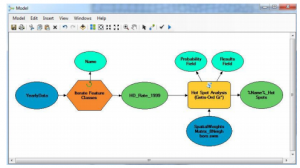
And the map it produced is next:
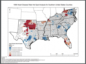
A high quality version can be found here: HotSpot Map
The map shows hot and cold spots of heart disease. The clusters were identified using a hotspot analysis which shows statistically significant clusters of high and low values.
Lab 2: Exploring FragStats
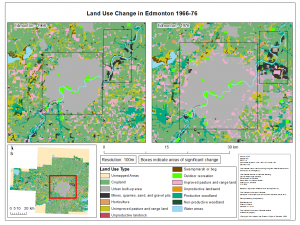
For this lab we were introduced to a program widely used in Landscape Ecology, FragStats. The goal of this lab was to carry out an analysis of land use change in Edmonton, Alberta using FragStats to analyze the specifics of how the land was changing. Things like Patchiness, Patch Diversity, and Land Use type were considered using the program and a transition matrix to see how specifically land in the Edmonton area was being changed. We were then asked to research the potential effects of our results as a consultant to the government.
For my analysis I chose to focus on the conversion of agricultural land surrounding Edmonton into urban or industrial land. Using Canada Land Use Monitoring Data from Geogratis the change of these lands was analyzed through FragStats, ArcMap, and Microsoft Excel. Through the analysis I found that from 1966-1976 there was a 280.58% change in the urban built up area around Edmonton resulting in an over 30,000 hectare increase in urban land coverage. With the knowledge that Edmonton had historically been converting agricultural land to urban land and continues to do so I had two main recommendations as a consultant:
- The establishment of agricultural zones of high importance similar to the Agricultural Land Reserve in Vancouver, B.C
- Establishment of defined urban growth boundaries to prevent loss of land and significant urban sprawl.
The maps showing this can be found below:
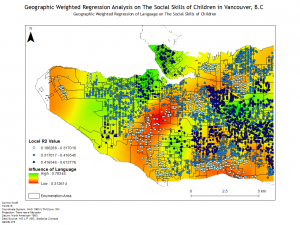
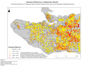
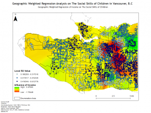
Lab 3: Geographically Weighted Regression
In this lab we were introduced to Geographically Weighted Regression which is a powerful spatial regression tool within ArcMap. To demonstrate the strength of this analytical process we conducted a regression analysis of childhood social scores in Vancouver, B.C. We conducted a series of regressions on social and demographic factors to determine the importance of them of social scores. We began by using an exploratory regression to determine the variables that had the largest impact on the social scores and then conducted an Ordinary Least Squares regression and a Geographically Weighted Regression. By performing both regressions we learned the difference between the two through the different results. An Ordinary Least Squares regression uses a global model while a Geographically Weighted Regression utilizes a local model which internalizes Tobler’s First Law which states “everything is related to everything else, but near things are more related than distant things.”
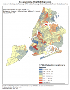
Geographically Weighted Regression proved to be a powerful tool for analyzing the spatial relationship of variables. I ended up using it for the final research paper of Urban Research 450 to carry out a study of the School to Prison Pipeline in New York City. Through the project I conducted both and Ordinary Least Squares Regression and a Geographically Weighted Regression and found that the local spatial relationships that contributed to the pipeline were enormous, with much higher r-squared values and consistent residuals found using the Geographically Weighted Regression.
Below are a few of the maps created for the lab and a map for Urban Research:
Lab 4: CrimeStat
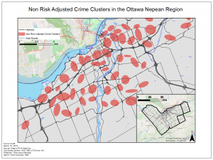
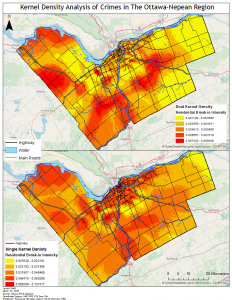
In this lab we explored the application of GIS in crime by using CrimeStat. To do this we analyzed crime patterns in the Ottawa- Neapan region of Ontario, Canada. Using Crime data for the area we looked at the spatial distribution of break and enters as well as car thefts. In CrimeStat we applied several analytical tools to our data, such as: a nearest neighbour spatial aggregation index, a Moran’s Index spatial autocorrelation correlogram, a fuzzy hotspot analysis, a nearest neighbour hierarchical clustering analysis, and a Knox index. Utilizing these methods the spatial distribution of crime in this area of Ontario was analyzed. I found that crime in this area was spatially autocorrelated and tended to cluster according to attributes such as property type and land use depending on the type of crime committed. Car thefts tended to occur in urban areas where a large number of cars would be parked throughout the day and residential break and enters tended to occur in heavily residential areas. Using the Knox index we added a temporal variable to our analysis of car thefts to find that car thefts were most likely to occur close in time but not in space suggesting these thefts occur at specific times of the day in a spree like fashion.
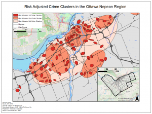
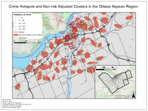
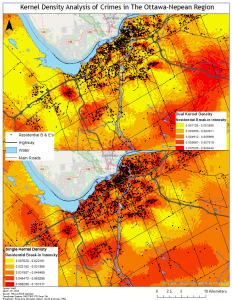
To further analyze the spatial distribution and risk of crime in the area a risk adjusted hotspot map as well as single and dual kernel density maps were created. The risk adjusted hotspot map adjusted for risk by adding population to the equation, normalizing crime by the amount of people to determine the risk of crime per person rather than a raw value. A single and dual kernel density map was then produced to analyze the intensity of crime across the area over a continuous surface. A kernel density map creates a continuous surface by interpolating values between points to create a map where the predicted intensity of crimes can be seen over the entire area. The single kernel density map showed the raw values of crime while, like the risk adjusted hotspot map, the dual kernel density map normalized the number of crimes against population. A few of the maps produced for this lab are below: