To provide a background for historical and projected climate trajectories at barkerville, I am doing a discriminant analysis on the geographical climate variability of the BEC variants along the Quesnel-Barkerville transect. This discriminant analysis creates a distinctive arch-shaped curve in the first two discriminating dimension, and a zig-zag in the third dimension (Figure 1). The arch shape is similar to the results from pilot project discriminant analysis of interannual variation at representative sites along the transect. The purpose of this blog is to answer: What is the meaning of these non-linearities in reduced climate space? Do they indicate a methodological problem?
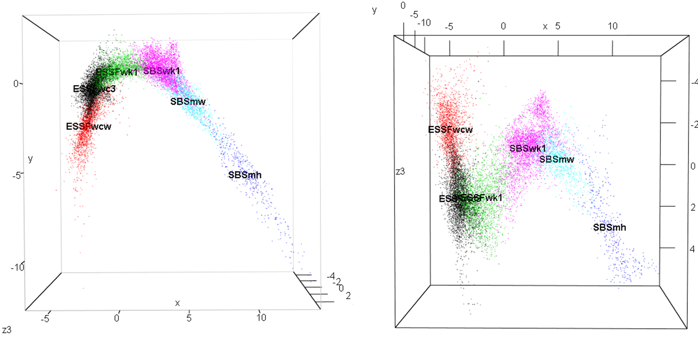
Figure 1: Biogeoclimatic variants of the Quesnel-Barkerville transect plotted in a 3-dimensional space created using discriminant analysis. Points are the ClimateBC 1961-1990 normals for 1600-m grid cells covering the geographic area of each variant. The points form an arch in the x-y plane (left) and a zig-zag in the x-z plane (right).
Hypothesis
The most likely explanation for these shapes are that they are an inevitable outcome of reducing the dimensionality of a climate space made up of variables with non-linear relationships to each other along a gradient. If all relationships were linear, climatic patterns in the gradient could be reduced to a multidimensional plane. Any two-dimensional representation (e.g. x-y, x-z, or y-z) of this plane would appear as a linear relationship, plus some noise. Indeed, if the linear relationships between the variables are correlated, then the first axis (first rotation) will capture all of these linear relationships, and all of the other axes will simply represent the noise in the rest of the dimensions. However, non-linear relationships between the variables will not be captured in this first rotation. It is likely that second-order non-linearities (arches) will be most common and therefore represented on the y axis. Third-order non-linearities (zigzags) would be captured in the third axis. This sequencing of non-linearities is evident in the Quesnel-Barkerville transect. Notably, the fourth axis contains a fourth order non-linearity.
Non linearities might also be the result of rotations that combine two or more variables that are static along a portion of the transect. Any non-linear variables that have discriminating variability on only one side of the first axis are possibly being combined on the second axis with uncorrelated variables that have discriminating variability on the other side of the first axis. This could also create an arch shape. An example of two variables that might create this effect are PAS and CMD. Both variables can be static (zero) along one extreme of the elevation range (Figure 2). Low elevation variants will be poorly discriminated by PAS, but highly discriminated by CMD. High elevation variants may have the opposite differentiating variables. it seems likely that both could be associated with a secondary discriminating axis, not because they are correlated, but because there is little overlap between the groups (variants) that they discriminate.
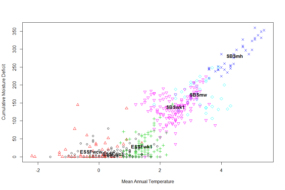
Figure 2: relationship of cumulative moisture deficit to mean annual temperature. CMD is an example of a variable that differentiates only a subset of the groups (BEC variants). It is static (zero) within most of the ESSF. This non-linearity cannot be resolved with a transformation.
Structure of the discriminant functions
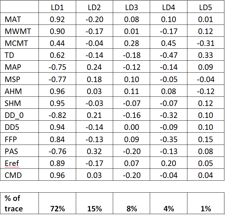
Despite the use of 14 climate variables, there are only five linear discriminating (LD) functions because there are only 6 BEC variant groups (Table 1). The first discriminating function accounts for 72% of the total separation achieved by the analysis, and almost all of the variables are highly correlated with this axis. This dominance of the first LD axis across all variables is expected because the groups are associated with an elevation gradient that strongly affects all variables. Winter variables have lowest correlation, which reflects the poor differentiation of BEC variants during the winter, as observed in previous analyses. The second and third axes both account for enough differentiation to be retained (>5% of trace). The first axis is clearly an index of dry/warm conditions. the second axis has no obvious intuitive climatic interpretation. However, it is notable in a scatterplot matrix (Figure 3) that the variables that are most highly correlated with LD2 (PAS, DD_0, MAP, MAT) have second-order nonlinearities with variables that are highly correlated with LD1 but highly uncorrelated with LD2 (CMD, AHM, SHM). Similarly, the variables that are most highly correlated with LD3 (MCMT, PAS, CMD, TD) have third-order nonlinearities with LD1 variables that are highly uncorrelated with LD3 (MWMT, DD5, SHM, Eref). This pattern supports the main hypothesis stated above, i.e. that the discriminant functions primarily reflect different types (orders) of non-linearities in the relationships between variables. The relationship of CMD to LD1 and LD2 indicates that the secondary hypothesis (presence of zero values along a portion of the gradient) is not a major factor in creating the arch.
- Table 1: structure coefficients of the discriminant functions. These are simply the correlations between the values of each observation on the discriminant functions with their original values on each climate variable.
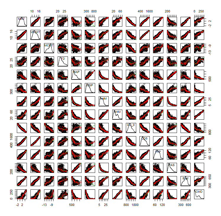
Figure 3: scatterplot matrix showing the pairwise relationships between individual climate variables.
Are log-linear transformations helpful?
Presumably, some of the non-linearities in the data are due to non-normal distributions in some of the variables. Transformation of these variables should therefore reduce the arch shape in the second dimension.
The discriminant analysis methodology and data used for the Quesnel-Barkerville transect analysis is largely derivative of Hamann and Wang (2006). These authors used a log10-transformation on precipitation and heat-moisture indices. Log10 transformations of these variables appear to be appropriate within the Quesnel-Barkerville BEC variants (Figure 4). The only exception is CMD, which should not be log-transformed due to the large number of zero observations. CMD was not included as an analysis variable in Hamann and Wang (2006). I am not clear on whether it was intentionally excluded, or simply not available in the early versions of ClimateBC used for that study.
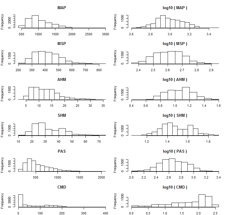
Figure 4: histograms of precipitation and heat-moisture indices over the geographic area of the six BEC variants of the Quesnel Barkerville transect.
Discriminant analysis using the transformed precipitation and heat-moisture variables increases the discriminating power (proportion of trace) of the first discriminating function by 7% (Table 2). Nevertheless, the arch relationship between LD1 and LD2 is graphically very similar to the analysis on the untransformed variables (Figure 5). This indicates that the skewed distributions in moisture variables contribute to the arch and zigzag shapes in LD2 and LD3, but that they are not solely responsible. This makes sense, since some temperature variables are correlated with LD2. Nevertheless, it is surprising that the arch shape remains so well preserved in the analysis of transformed variables.
Table 2: Proportion of trace for the discriminant functions (axes) with transformed and untransformed moisture-related variables. This metric describes the amount of the total differentiation achieved by the analysis that is attributable to each discriminant function.
|
LD1 |
LD2 |
LD3 |
LD4 |
LD5 |
|
| untransformed |
72% |
15% |
8% |
4% |
1% |
| transformed |
79% |
13% |
4% |
3% |
1% |
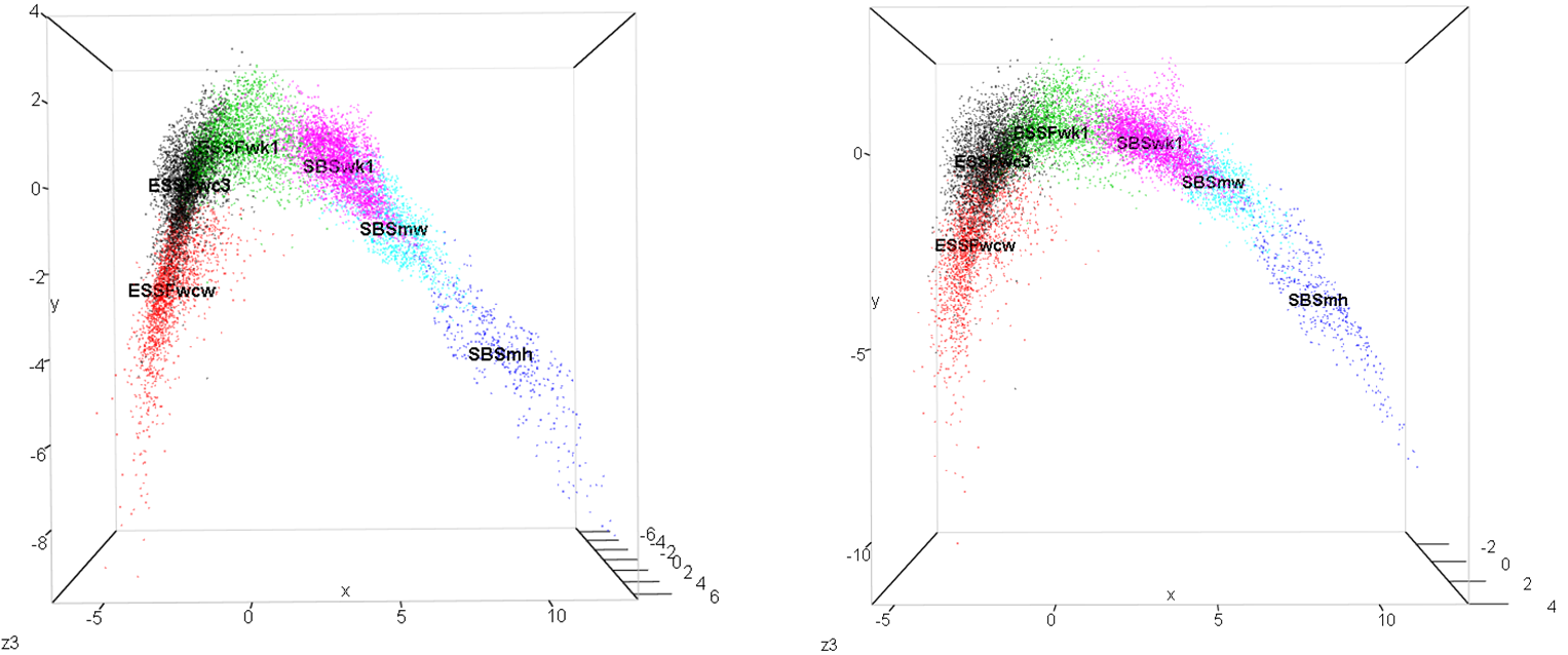
Figure 5: comparison of the first two discriminant axes of the Quesnel-Barkerville BEC variants using untransformed (left) and log-10 transformed (right) precipitation and heat moisture variables (MAP, MSP, PAS, AHM, and SHM).
Is this the arch or horseshoe effect?
Superficially, this situation resembles the arch effect and horseshoe effect that frequently occurs in multivariate analysis of plant communities along environmental gradients. The horseshoe effect is generally regarded as a fatal flaw for use of PCA with species occurrence data in which species have a unimodal response curve to an environmental gradient . The gaussian response curves of each plant species overlap along the gradient, meaning that the species are non-linearly related to each other in species space. This is the cause for the arch effect. In addition, PCA may incorrectly portray sites on the opposite sides of the environmental gradient as being closely related due to a large number of shared species absences at these sites. This causes the ends of the arch to become incurved, and confounds interpretation of the principle components. This situation is called the “horseshoe effect”. Michael Palmer provides a good summary of the horseshoe effect and its causes (http://ordination.okstate.edu/PCA.htm).
Arch effects have been noted in principal components analysis (PCA), correspondence analysis (CoA), principal coordinates analysis (PCoA) and non- metric multidimensional scaling (NMDS) (Podani and Miklos 2002). I couldn’t find any reference to the arch or horseshoe effect in the context of discriminant analysis, but I’m also not aware of a reason that the same principles wouldn’t apply to discriminant analysis. Podani and Miklos (2002) make the important and obvious point that “whereas unimodal species response to long gradients always leads to horseshoe (or arch)-shaped configurations in the first two dimensions, the converse is not true; curvilinear arrangements cannot generally be explained by the Gaussian model.” The climate variables making up the climate space in the Quesnel-Barkerville transect do not have Gaussian distributions along the elevation/temperature gradient. More generally, they never have zero values at both ends of the gradient. For this reason, there is no reason to believe that the arch shape displayed in the first two discriminant axes is the “arch effect” commonly observed in species space.
Conclusions
This informal investigation appears to have explained the reason for the second-order (arch) and third-order (zig-zag) non-linearities in the second and third discriminating functions for the Quesnel-Barkerville BEC variants. the discriminant functions appear to primarily reflect different types (orders) of non-linearities in the relationships between climate variables, rather than functional differences in individual variables. this is a logical, and possibly inevitable, result of doing discriminant analysis on groups that are sequentially located along an environmental gradient. This is an important result, because functional differences in climate variables are often sought during interpretation of the meaning of discriminating functions. In this case, functional differences between variables are a secondary consideration. It is unclear how the effect observed on this environmental gradient will play out over larger and more complex sets of BEC variants. Investigating this effect over a broader geographic scale (e.g. all BEC variants of the BC coast) is an important next step.
Climate variables with limits at zero (e.g. CMD) may create non-linearities in the reduced-dimensional climate spaces. However, no major problems were evident from this cursory analysis. The implications of zero-limited variables (e.g. CMD) for discriminant analysis should be investigated.
References
Hamann, A., and T. Wang. 2006. Potential Effects of Climate Change on Ecosystem and Tree Species Distribution in British Columbia. Ecology 87:2773–2786.
Podani, J., and I. Miklos. 2002. Resemblance coefficients and the horseshoe effect in principal coordinates analysis. Ecology 83:3331–3343.
R Code
###R code for Blog 1 (Sept29, 2013) "Non-linearities in reduced-dimension climate spaces along a climatic gradient"
##investigate non-linearities in the linear discriminant analysis of the Quesnel-Barkerville BEC variants
#Read in the ClimateBC 1961-90 Normals on the 1600-m grid provided by Tongli.
mydata <- read.csv("C:\\Users\\Colin\\Documents\\Masters\\Research\\Data\\ClimateBC\\BEC7v      1600_QuesBark_Normal_1961_1990Y.csv", strip.white = TRUE, na.strings = c("NA","") )
mydata <- mydata[-(which(mydata$MAT==-9999)),]
colnames(mydata)[1]<-"id400"
colnames(mydata)[2]<-"var"
mydata$var<-gsub(" ","", mydata$var , fixed=TRUE) #strip white space
VarList<-data.frame(var=as.character(levels(factor(mydata$var))),
      count=as.vector(table(mydata$var)))
#Remove irrelevant and collinear variables
mydata$DD_18<-NULL #remove heating degree days (irrelevant)
mydata$DD18<-NULL #remove cooling degree days (irrelevant)
mydata$NFFD<-NULL #very highly collinear with FFP
mydata$bFFP<-NULL #very highly collinear with FFP
mydata$eFFP<-NULL #very highly collinear with FFP
mydata$EMT<-NULL #not very relevant
mydata$EXT<-NULL #very highly collinear with MCMT and not very relevant
##histograms of untransformed and transformed variables
par(mfrow=c(6,2))
par(mar=c(2,4,4,1))
hist(mydata[,10], main=colnames(mydata)[10])
hist(log10(mydata[,10]), main=paste("log10 (",colnames(mydata)[10],")"))
hist(mydata[,11], main=colnames(mydata)[11])
hist(log10(mydata[,11]), main=paste("log10 (",colnames(mydata)[11],")"))
hist(mydata[,12], main=colnames(mydata)[12])
hist(log10(mydata[,12]), main=paste("log10 (",colnames(mydata)[12],")"))
hist(mydata[,13], main=colnames(mydata)[13])
hist(log10(mydata[,13]), main=paste("log10 (",colnames(mydata)[13],")"))
hist(mydata[,17], main=colnames(mydata)[17])
hist(log10(mydata[,17]), main=paste("log10 (",colnames(mydata)[17],")"))
hist(mydata[,19], main=colnames(mydata)[19])
hist(log10(mydata[,19]), main=paste("log10 (",colnames(mydata)[19],")"))
par(mfrow=c(1,1))
par(mar=c(4,4,2,2))
#Pairs plot of x variables, using an N=500 random subsample to avoid overplotting
mysample <- mydata[sample(1:nrow(mydata), 500, replace=FALSE),]
library("car")
scatterplotMatrix((mysample[,6:length(mysample)]))
#
x <- mysample$MAT
y <- mysample$CMD
xhat<-tapply(x, INDEX = mysample$var, FUN = mean, na.rm=TRUE)
yhat<-tapply(y, INDEX = mysample$var, FUN = mean, na.rm=TRUE)
plot(x,y,col=as.numeric(factor(mysample$var)), pch = as.numeric(factor(mysample$var)),
 xlab = "Mean Annual Temperature", ylab = "Cumulative Moisture Deficit (CMD)",
 main="")
text(xhat, yhat, levels(factor(mysample$var)), font=2)
library(MASS) #contains lda; also eqscplot(x,y) function, which plots axes of equal scale
library(stats)
#define the matrix of x variables
X<- mydata[,6:length(mydata)]
#transform the 5 precip and heat-moisture variables (optional).
#X$MAP <- log10(mydata$MAP)
#X$MSP <- log10(mydata$MSP)
#X$AHM <- log10(mydata$AHM)
#X$SHM <- log10(mydata$SHM)
#X$PAS <- log10(mydata$PAS)
##MDA
z <- lda(X, mydata$var)
##Data frame of discriminant axis scores
M <- as.data.frame(predict(z)$x )
##Plot of BEC variants on first two discriminant axes
x<-M[,1]
y<-M[,2]
z3 <- M[,3]
A<-factor(mydata$var) #points are labelled by mapped bec variant.
variant<-"ESSFwk1"
# Spinning 3d Scatterplot
library(rgl)
#?plot3d
#?rgl
plot3d(x, y, z3,
 col = as.numeric(factor(A)),
 alpha = 0.5,
 ylim=c(0.1,max(y)),
 zlim=c(0.1,max(z3)),
 size=2)
##Labels at the 3D psuedocentroid
xhat<-tapply(x, INDEX = mydata$var, FUN = mean, na.rm=TRUE)
yhat<-tapply(y, INDEX = mydata$var, FUN = mean, na.rm=TRUE)
z3hat<-tapply(z3, INDEX = mydata$var, FUN = mean, na.rm=TRUE)
text3d(xhat, yhat, z3hat, text = levels(factor(A)), font=2)
######################Quantitative Analyses
##Structure coefficients
 #Correlations between predictors and discriminant values
 #indicate which predictor is most related to discriminant function (not corrected for the            #other variables)
CorXM <- cor(X,M)
write.csv(CorXM, "C:\\Users\\Colin\\Documents\\Masters\\Research\\Data\\CorXM.csv")
##Basic descriptive output for the LDA
#the singular value decomposition gives the ratios of the between- and within-group
         #standard deviations on the linear discriminant variables.
z
z$svd
