Summary

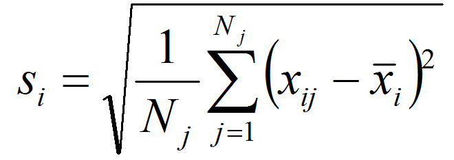
A meaningful metric of climatic difference is helpful for climate change analysis. There is a strong statistical and ecological rationale for the use of Mahalanobis metrics in multivariate analysis of climatic novelties, since it removes the effect of correlations and trivial redundancies between climate variables. This post describes standardization of eigenvectors on the temporal component of spatiotemporal data. In other words, this method performs a second round of spatiotemporal standardization on features extracted from spatiotemporally standardized data.  This second standardization approach appears to be functionally (and possibly mathematically) equivalent to spherical normalization of the within-groups covariance matrix of extracted features, which is commonly used within linear discriminant analysis to improve classification. In addition to its advantages in classification, this method provides a Mahalanobis metric whose units reflect the average temporal variability of the study area. This “M-metric” is a robust and ecologically meaningful metric for quantification of climatic differentiation and change.

The rationale for standardization of extracted features

Standardization (a.k.a. scaling) is a very common procedure in multivariate analysis. The basic rationale for standardization is that different variables have different and incomparable units of measurement (e.g. ^oC vs. mm). However, even for variables with comparable units, there is an additional ecological rationale for standardization of interannual variability: life strategies of organisms will generally be adapted to the background variability of any given climate element. Adaptation to historical variability is expected to be both temporal (e.g. winter vs. summer temperatures) and spatial (e.g. mean annual temperature in temperate vs. tropical regions) (Mora et al. 2013). This ecological rationale for standardization must be considered in metrics for climatic differences in both space and time.

Standardization gives all variables equal or comparable variance, and thus equal a priori influence on the outcome of a principle components analysis (PCA). However, PCA aggregates the correlated variance of the raw variables into the extracted principal components. The relative variance of the principal components thus reflects the redundant variance in the raw variables. Addition of a trivially and perfectly redundant variable to the raw data (e.g. a second set of MAT values), will have the non-trivial result of increasing the variance of one of the principal components and possibly increasing its rank. This behaviour highlights the importance of careful variable selection prior to performing PCA. Nevertheless, correlation between raw climate variables is inevitable, and so the ecological meaning of the unequal variance of principal components needs to be considered.

Extracted features (e.g. principal components) represent independent (uncorrelated) dimensions of climatic variation. Regardless of whether unequal variance in the principal components is due to trivial redundancies or meaningful correlations, the relative scales of variation in the principal components are unlikely to be ecologically meaningful due to life strategy adaptation.  What is important is the magnitude of a climatic difference or change relative to the background variation of any given principal component. In this light, the ecological rationale for standardization of raw variables also applies to principal components and other eigenvectors extracted by other methods, such as LDA.

Mahalanobis distance vs. Euclidian distance

I have demonstrated in previous posts that principal components analysis doesn’t affect the distance between observations in climate space. Therefore, Euclidian distance on non-truncated principal components is the same as Euclidian distance on raw variables. Standardization of the principal components (dividing by the standard deviation of z-scores) creates a climate space in which Euclidean distance is equivalent to Mahalanobis distance in the standardized but unrotated climate space (Stephenson 1997).  The units of standardized eigenvectors (e.g. standardized principal components) therefore are Mahalanobis metrics. Similar to z-scores, the precise meaning of a Mahalanobis metric depends on how the eigenvectors are derived from the raw data (e.g. PCA vs. LDA) and how the standardization population is defined (e.g. global vs. spatiotemporal).

Spherization of temporal climate envelopes

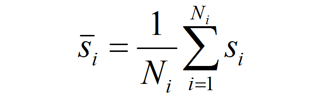
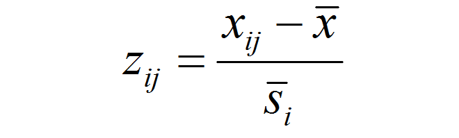
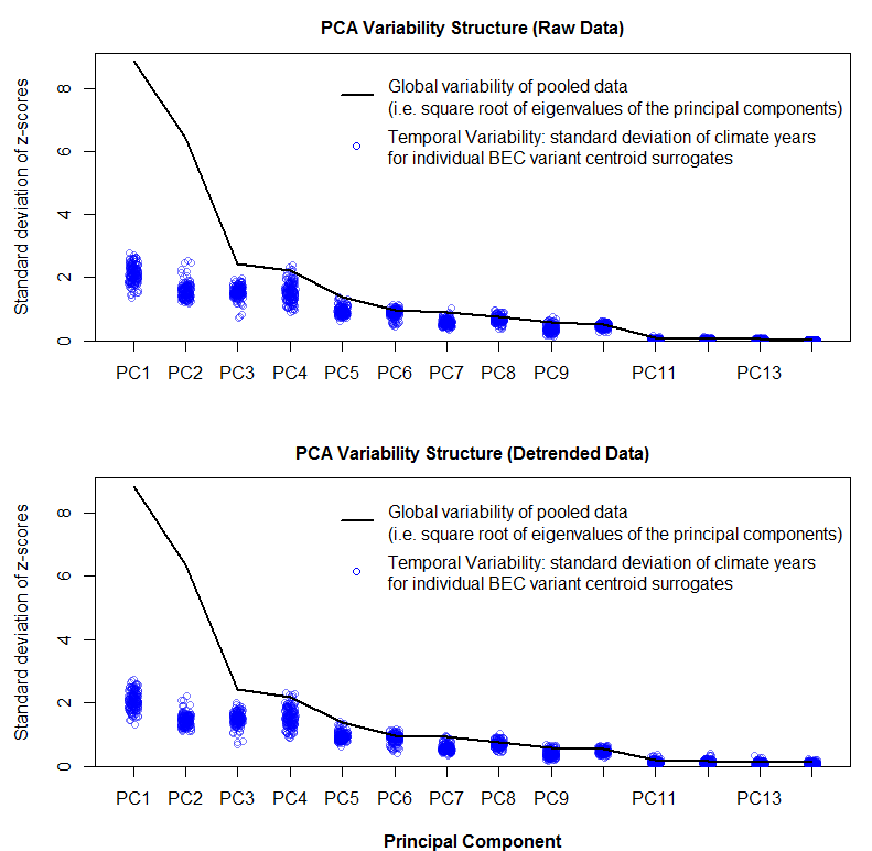
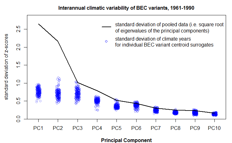
As shown in the previous post, spatiotemporal standardization operates by dividing each observation by the average standard deviation of climatic anomalies across the study area. This approach creates temporal climatic envelopes that are approximately spherical, and collectively have an average standard deviation of one z-score. Climate envelopes of individual locations will be larger or smaller, and more-or-less spherical, depending on their variability in each climate element relative to the study area average. Principal components analysis of this space is desirable, since it aggregates redundant variation into uncorrelated dimensions of variation. However, the aggregation of variance into principal components creates ellipsoidal (oblong) temporal climate envelopes. As discussed above, the ecological meaning ellipsoidal shapes of temporal climate envelope is ambiguous.  A second round of spatiotemporal standardization of the principal components returns the temporal climate envelopes to an approximately spherical shape. This second standardization can be called “spherization of within-group variability,” or just “spherization” for simplicity.  The metric of the sphered climate space can be called the M-score, because it represents a unit of Mahalanobis distance based on the average standard deviation of temporal anomalies of z-scores over all locations in the study area. The process of spherization of truncated principal components is illustrated in Figure 1.

Figure 1: effect of spatiotemporal standardization of principal components (spherization) on the variability structure of the BEC variants of the south-central interior BC.

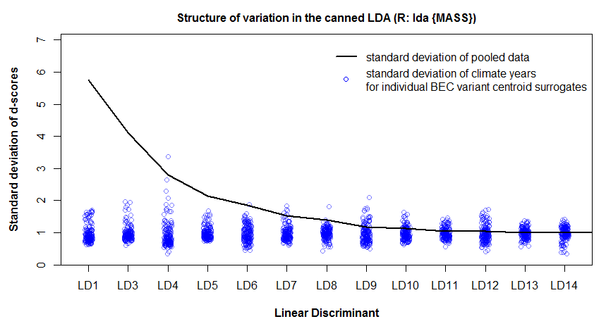
Figure 2: the role of spherization in linear discriminant analysis of the BEC variants of the south-central interior BC.

Comparison with linear discriminant analysis

Many aspects of the above procedure (spherization of local anomalies (within-group variability) of the principal components of spatiotemporally standardized data) are conceptually similar to the procedures of linear discriminant analysis. A comparison of the methods and results of the two procedures is warranted.

Spatiotemporal standardization expresses spatial variability between locations in terms of the average temporal variability of all locations. This is similar, though not equivalent, to the ratio of between-groups to within-groups scatter matrix that is the basis of LDA: The within-groups scatter matrix is the sum of the individual group covariance matrices, which is equivalent to the average covariance matrix, which in turn is likely equivalent in ratio form to the average matrix of standard deviations.  Variables that have higher spatial variability will have larger variance in a spatiotemporally standardized data set. A principal components analysis of spatiotemporally standardized data is therefore functionally similar to LDA, because both give high priority (eigenvalues) to variables with a high ratio of between-group to within-group variability.

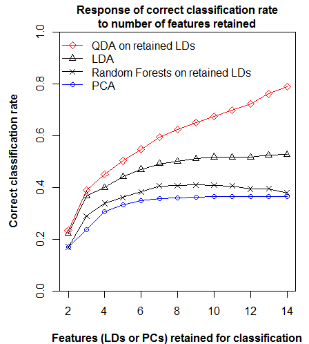
Despite this functional similarity, PCA calculates eigenvalues of the total data variance, while LDA calculates eigenvalues of the ratios of between- to within-group variance. The extracted features are different as a result. Low-eigenvalues in PCA indicate residual dimensions with very low spatial and temporal variation (Figure 1).  Low eigenvalues in LDA indicate dimensions with low spatial variation, but which may nevertheless have substantial temporal variability (Figure 2). PCA is advantageous because it facilitates truncation of the features with very low variance; in Figure 1 it is clear that the last four principal components can be dropped from further analysis with minimal loss of information. However, beyond the process of truncation, the advantages of PCA vs. LDA are ambiguous. PCA structures the climate space in order of decreasing total variance, while LDA structures the climate space in order of decreasing spatial differentiation. Both of these structures are climatically and ecologically meaningful in their own way, and their relative advantages will depend on the specific research question being asked.

Effect of spherization on climate year classification

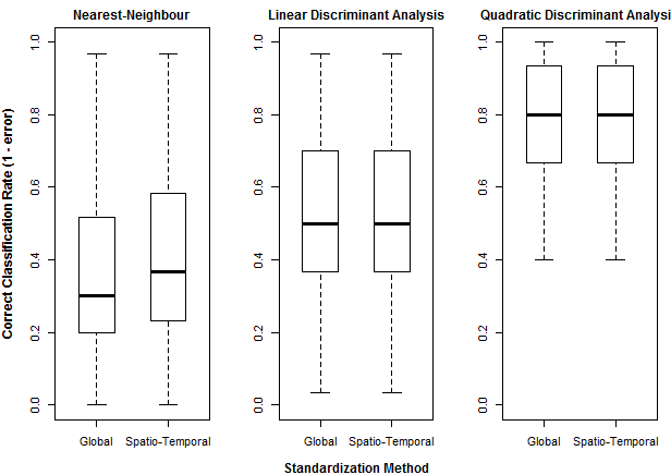
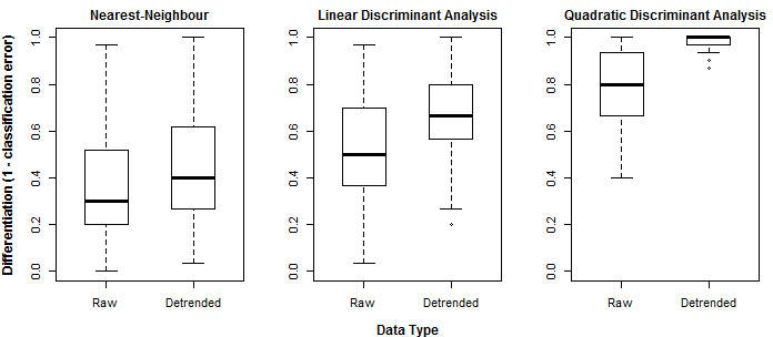
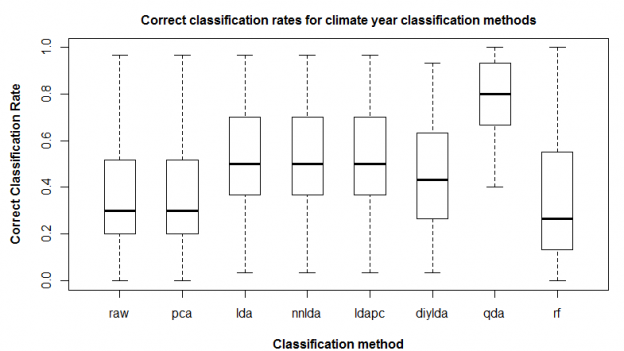
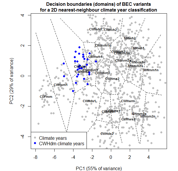
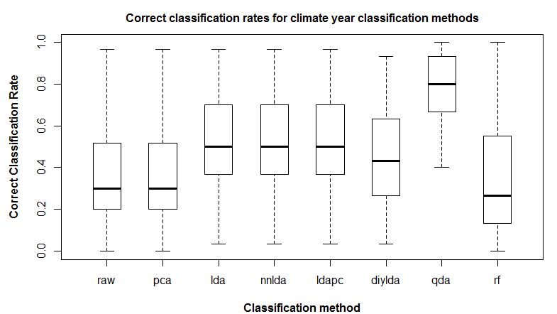
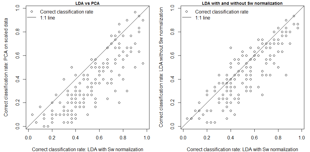
Spherization is not integral to the feature extraction component of the LDA procedure, but it is typically incorporated into LDA because it has an important role in classification. For example, it is an integral component of the lda{MASS} call in R. it is logical that spherization of the principal components should also improve nearest neighbour classification. Figure 3 demonstrates the sequential effects of spatiotemporal standardization and spherization on differentiation (nearest-neighbour correct classification rates) between BEC variant temporal climate envelopes. Typical global z-standardization produces an average differentiation in the otherwise untransformed climate space of 36%. Spatiotemporal standardization improves differentiation to 41%. As demonstrated previously, PCA has no effect on differentiation. However, spherization of the PCA improves differentiation to 47%. LDA, which includes spherization as part of its classification procedure, achieves a differentiation of 53%. It is notable that LDA without spherization (not shown in Figure 3) only achieves 44% differentiation. Spherization is clearly advantageous for classification. Spatiotemporal standardization followed by spherization of principal components achieves classification results that are only marginally poorer than LDA.

Figure 3: effect of spatiotemporal (ST) standardization and spherization on climate year classification of BEC variants, compared to simple “global” z-standardization (left) and linear discriminant analysis (LDA, right). All classifications use the nearest-neighbour criterion.

Use of spherization and Mahalanobis distance in the ecological literature climate change

Standardized anomalies are frequently used in the atmospheric sciences , and are useful for univariate analysis because they quantify variability in terms of standard deviations (z-scores). Mora et al. (2013) adapted the concept of standardized anomalies to describe “climate departures”, i.e. the year at which the future temporal climate envelope of any given location ceases to overlap with its own historical temporal climate envelope. Although they did univariate analysis on seven climate variables, they did not perform any multivariate analysis. This is very likely due to the purpose of their paper as a simple way to communicate climate change impacts to a large non-expert audience. Nevertheless, the high impact of this paper suggests that an equivalent multivariate approach is in demand.

Williams et al. (2007) provided a multivariate analysis of standardized anomalies, using a standardized Euclidean distance metric. The authors may have opted against a Mahalanobis metric for the sake of simplicity and ease of communication.  Nevertheless, standardized Euclidean distance metrics are susceptible to the unjustified influence of correlations in the input variables, and so are problematic for quantitative investigation of climate change.

Hamann and Wang (2006) used linear discriminant analysis on spatial variation in climate normals to define the climate envelopes of BEC variants for the purposes of climate change analysis. They explicitly noted that this method uses a Mahalanobis distance for climatic classification. This Mahalanobis metric is very similar to the one I have proposed because it is based on spherization of within-group variability. However, the units of the Mahalanobis metric in Hamann and Wang (2006) reflect the average spatial variation of climate normals within BEC variants, and thus the scale of BEC mapping. A Mahalanobis metric based on the temporal variation at individual locations is essentially independent of BEC mapping, which is likely preferable for subsequent analysis of BEC mapping.

As an alternative to discriminant analysis for species distribution modeling, Roberts and Hamann (2012) proposed nearest-neighbour classification using Euclidean distance of heavily truncated principal components. They claimed that this is a modified Mahalanobis distance, but do not specify any standardization of the principal components in their methodology. Euclidian distance on principal components is the same as Euclidian distance on raw variables. As a result, it does not appear that their method produces a Mahalanobis metric, though this needs to be verified.

References

Hamann, A., and T. Wang. 2006. Potential Effects of Climate Change on Ecosystem and Tree Species Distribution in British Columbia. Ecology 87:2773–2786.

Mora, C., A. G. Frazier, R. J. Longman, R. S. Dacks, M. M. Walton, E. J. Tong, J. J. Sanchez, L. R. Kaiser, Y. O. Stender, J. M. Anderson, C. M. Ambrosino, I. Fernandez-Silva, L. M. Giuseffi, and T. W. Giambelluca. 2013. The projected timing of climate departure from recent variability. Nature 502:183–7.

Roberts, D. R., and A. Hamann. 2012. Method selection for species distribution modelling: are temporally or spatially independent evaluations necessary? Ecography 35:792–802.

Stephenson, D. B. 1997. Correlation of spatial climate/weather maps and the advantages of using the Mahalanobis metric in predictions. Tellus 49A:513–527.

Williams, J. W., S. T. Jackson, and J. E. Kutzbach. 2007. Projected distributions of novel and disappearing climates by 2100 AD. Proceedings of the National Academy of Sciences of the United States of America 104:5738–42.

Summary

This post describes a modification of anomaly standardization for spatiotemporal climate data. I have not yet found an explicit description of this approach in the literature, so for the moment I am calling it spatiotemporal standardization. This method standardizes climate variables by the average standard deviation of interannual variability of all locations in the study area. It is a useful compromise between typical “global” z-standardization across the whole data set and anomaly standardization of each location’s interannual variability. Spatiotemporal standardization serves two important purposes for climate change analysis: (1) it provides an ecologically meaningful metric of climatic difference—the spatiotemporal z-score—that directly reflects observed interannual variability in each climate element; and (2) it supports PCA feature extraction that appropriately balances spatial (between-group) and temporal (within-group) variability. Unlike local anomaly standardization, spatiotemporal standardization does not distort the climate space: it preserves the relative distances between all observations within any given variable. However, it alters euclidean distance of the climate space by emphasizing variables with high spatial (between-group) variability, and therefore improves climate year classification results. Spatiotemporal standardization appears to be an effective foundation for analysis of bioclimate differentiation, historical variability, and degrees of climatic novelty.

Global, anomaly, and spatio-temporal standardization

Standardization is necessary for multivariate analysis of climate data because climatic elements (e.g. temperature and precipitation) have different units and scales (e.g. degrees Celsius and millimetres). Z-standardization subtracts the population mean from each observation, and then divides by the population standard deviation. This method reduces observations to z-scores, which have a mean of zero and unitless values representing standard deviations above and below the mean. Beyond the simple utility of standardization, the z-score is a useful concept for climatic analysis because it provides a metric of climatic difference that is directly related to the statistical variability of climate elements.

The z-standardization process can be customized for specific purposes by carefully defining the population.  The most common approach to z-standardization is to treat all observations in the data as one population. This approach can be called “global standardization”. The major disadvantage of global standardization for spatio-temporal data sets is that it returns z-scores that arbitrarily reflect the spatial variation of climate elements over the study area (a larger study area will have a larger range of variation), and which therefore have limited ecological meaning. An alternate approach is to apply standardization locally and temporally by defining the population as the annual observations at one location over a given time period. This is called anomaly standardization in the atmospheric sciences. Standardized anomaly z-scores are a measure of climatic difference in space or time in terms of the historical range of climatic variability at an individual location. Standardized anomalies thus provide an ecologically meaningful metric for climatic differences between locations, for the magnitude of climate change, and for analog goodness-of-fit. For example, anomaly standardization is the basis for the “standardized Euclidian distance” approach described by Williams et al. (2007) for their analysis of novel and disappearing climates.

One limitation of anomaly standardization is that it transforms climate data at each location by a different scalar, and therefore distorts the spatial structure of temporal variability in the study area. This removes important information from the data and precludes comparison of the relative magnitude of historical variability and future climate change at different locations. One solution to this problem is to standardize observations by the mean of the anomaly standard deviations in all locations of the study area. This approach is simple enough that it very likely has been previously developed. However, I haven’t yet found an explicit description in the literature. For the moment, I am calling it “spatio-temporal standardization” because it provides z-scores based on temporal variability that nevertheless preserve the spatial structure of variability in the data.

Explicit description of spatiotemporal standardization

For a spatiotemporal variable composed of j time series observations at each of i locations, the standard deviation of anomalies at each location i is:

The mean anomaly standard deviation over all i locations is:

Each observation x_ij is spatiotemporally standardized to a unitless score z_ij by subtracting the grand mean of the variable, and dividing by the mean anomaly standard deviation:

Effect of spatio-temporal standardization on PCA feature extraction

In previous blog posts I found that PCA of globally standardized climate data was problematic because it allowed variables with large interannual (within-group) variability to dominate the climate space, even if there was relatively little spatial (between-group) variability. This was exemplified in climate space of south-central BC, where variables associated with winter temperatures (TD and MCMT) dominated the second principal component. This type of high within-group and low between-group variability is unlikely to be ecologically important, because organismal life strategies are adapted to it (e.g. via dormancy in plants). Discriminant analysis is designed to address this problematic type of variability, but I found that it goes too far: LDA extracts features only on the basis of the ratio of between- to within-group variability, regardless of whether those features are important to the overall spatiotemporal variability of the study area. A compromise between PCA and LDA is required.

Spatio-temporal standardization provides an effective approach to balancing within-group and between-group variability in feature extraction. By standardizing on average temporal variability of the study area, climate elements are given equal emphasis relative to each other at any given location. This is ecologically justified, since organismal life strategies can be expected to be adapted to the general scale of variability in each climate element at any given location. A PCA of spatiotemporally standardized data will then emphasize climate elements with high spatial variability.

Figure 1: biplots of the first two principal components of globally standardized and spatiotemporally standardized climate data for the BEC variants of south-central interior British Columbia (BG, PP, IDF, ICH, SBS, SBPS, MS, and ESSF BEC zones). Red arrows indicate correlations between the two PCs and the 14 standardized climate variables.

The difference between PCA on globally standardized and spatiotemporally standardized data is illustrated in biplots of reduced climate spaces for south-central interior BC (Figure 1). Winter temperature variables TD and MCMT dominate PC2 in the globally standardized data because of their high within-group variability. Spatiotemporal standardization leads to much better differentiation of BEC variants in PC2. Variability structure plots (Figure 2) indicate that the winter temperature feature is shifted from PC2 in the globally standardized data to PC4 in the spatiotemporally standardized data.

Figure 2: structure of variability in principal components of globally standardized and spatiotemporally standardized climate data for the BEC variants of south-central interior British Columbia (BG, PP, IDF, ICH, SBS, SBPS, MS, and ESSF BEC zones).

Effect of spatio-temporal standardization on climate-year classification

Spatio-temporal standardization performs centering and scaling by coefficients that are common to all observations of any given variable. Nevertheless, the relative scaling of the variables changes, which changes the relative importance of the variables in contributing to Euclidian distance measures.  spatiotemporal standardization uses a denominator of temporal (within-group) variability. As a result, Euclidian metrics of spatiotemporally standardized data will emphasize variables with a high spatial (between-group) variation relative to temporal variation. As a result, it is logical that spatio-temporal standardization will improve nearest-neighbour classification. This effect is demonstrated in climate year classifications of BEC variants on globally vs. spatiotemporally standardized data (Figure 3). In this example, spatiotemporal standardization increases nearest-neighbour climate year differentiation from 36% to 41%. However, spatiotemporal standardization has no effect on LDA or QDA classification, since these methods include standardization procedures that override the a priori scaling of the input data.

Figure 3: comparison of climate year classification rates for globally and spatiotemporally standardized data.

References

Williams, J. W., S. T. Jackson, and J. E. Kutzbach. 2007. Projected distributions of novel and disappearing climates by 2100 AD. Proceedings of the National Academy of Sciences of the United States of America 104:5738–42.

Summary

Climate change trends must be removed from the interannual variability used to determine temporal climate envelopes, otherwise locations with rapid historical climate change would be interpreted as having greater background variability. However, the climate system is too complex to expect that there will be an objective division between trend and variability; an arbitrary distinction must be made. Empirical mode decomposition (EMD) (Huang et al. 1998) extracts intrinsic and adaptive trends from non-linear and non-stationary time series. In contrast to other intrinsic/adaptive methods such as locally weighted regression, EMD is appealing because it is the implementation of an explicit definition of trend. The results from this evaluation suggest that EMD is a viable method for removing the trend from historical climatic variability, though further refinement and testing are required to ensure that it is implemented appropriately. Detrending is shown to have a dramatic effect on climate year classification: there appears to be almost no overlaps in detrended climate envelopes of BEC variants. 

Figure 1: A time series of mean annual temperature in British Columbia’s central interior plateau. The differentiation of interannual variability from the long term climate change trend is not straightforward.

Distinguishing trend from variability

The premise of the temporal climate envelope approach is that interannual climatic variability at any given location provides a scale for assessing the ecological significance of climate change in both space and time. However, this approach requires that a distinction must be made between interannual variability and climate change. In order for the interannual variability to be quantified, the climate change trend must be removed. The methodology for removal of the trend can be a critical consideration for climate change analysis, because it implicitly defines what will be considered climate change as opposed to background variability.

The time series of mean annual temperature in British Columbia’s central interior plateau (Figure 1) demonstrates that detrending is essential to analysis of interannual variability. Without detrending, regions with more rapid historical climate change will be spuriously assigned a higher range of interannual climatic variability than regions with less historical climate change. This would confound an assessment of the ecological significance of climate change based on historical variability. However, the MAT time series suggests that there is no clear distinction between interannual variability and long term climate change. Oscillations are apparent, but they occur on a continuum of magnitudes and frequencies.

Wu et al. (2007) provide an excellent characterization of the problem of trend identification in climate data. They first explicitly define the term trend as an attribute specific to an arbitrary time scale: “The trend is an intrinsically fitted monotonic function or a function in which there can be at most one extremum within a given data span.” Their definition of variability follows: “the variability is the residue of the data after the removal of the trend within a given data span.”

They note that due to the complexity of the global climate system, climate time series must be expected to be non-linear and non-stationary. in light of this expectation, Wu et al. (2007) make a distinction between extrinsic/predetermined methods for trend identification and intrinsic/adaptive methods. Extrinsic methods—including linear and non-linear regression, classical decomposition, and moving averages—impose a predetermined functional form onto the data and therefore are inappropriate for nonlinear non-stationary time series.  Wu et al. (2007) advocate for intrinsic methods that are adaptive to the changing attributes of the signal throughout the time series. Specifically, they suggest empirical mode decomposition (EMD) (Huang et al. 1998) as the only method able to adequately determine the trend in nonlinear non-stationary time series.

Empirical mode decomposition (EMD)

EMD decomposes time series into intrinsic mode functions (IMFs), which are oscillations of various time scales that (1) have extrema and zero-crossings that differ in number only by one, and (2) have equal absolute mean values of minima and maxima. The residual of this process is a monotonic function with only one set of extremes, which is the trend as they previously defined it. EMD is an appealing approach for detrending variability. It is very widely cited (3320 citations in web of science), and deserves evaluation.

Figure 2:A demonstration of empirical mode decomposition (EMD) on the SBSwk3 MAT time series. This process was performed using the emd(y,x) command in R, with default parameters.

Figure 2 is a demonstration of EMD on the SBSwk3 MAT time series, using the emd(y,x) call in R with default parameters. There are some problematic features of the decomposition. For example, the prominent oscillation in the raw data from 1998 onwards seems to be very poorly decomposed: the removal of the first IMF puts subsequent IMFs out of phase and out of scale with this oscillation. This is likely an example of “mode-mixing”, which is cited as a common problem with EMD. However, the residual trend does not appear to be affected. Another potential critique of the residual trend is that it is out of phase with the dominant oscillation between 1950 and 1970. However, this is consistent with the explicit definition of trend in Wu et al. (2007); i.e. that a trend is a monotonic attribute of a given time span. Any oscillations over shorter time periods are explicitly considered be variability. This highlights the importance of choosing a time span that is meaningful to the interpretation of the variability and the trend.

EMD provides reasonable trend extraction over the 14 annual climate variables that I am currently using for my research (Figure 3). The EMD trends are similar to locally weighted linear regression (LOWESS), which is also an intrinsic/adaptive means of trend extraction. The main advantage of EMD over LOWESS is that EMD implements an explicit definition of trend that is free of local influences. However, EMD exhibits undesirable behaviour in the time series of mean summer precipitation (MSP), where it appears to exaggerate a very subtle trend. This undesirable behaviour appears to be primarily limited to the beginning and end of the time series.  For this reason, it is likely necessary to exclude some outer portion of the time span from the temporal climate envelope. Further exploratory work is required to ensure that I am implementing the method to its full potential.

Figure 3: Trends extracted by EMD from the time series of 14 annual climate variables at the SBSwk3 centroid surrogate. Another intrinsic/adaptive trend extraction, LOWESS, is shown for comparison.

Effect of detrending on climate-year classification

Detrending reduces the interannual variability at any given location, and therefore will reduce overlaps of temporal climate envelopes. As a result, it is logical that detrending will improve differentiation of BEC variants in a climate year classification. This effect is demonstrated in Figure 4. Notably, quadratic discriminant analysis achieves almost perfect differentiation on the detrended data (97% correct classification rate on average). This is a remarkable result, given that preliminary results using linear discriminant analysis on raw data suggested that there was approximately 50% overlap in BEC variant temporal climate envelopes. Since quadratic discriminant analysis classifies based on decision boundaries, the classification of detrended data indicates that there is almost no overlap in BEC variant temporal climate envelopes.

Figure 4: Effect of detrending on climate year classification results for the 1961-1990 normal period.

Effect of detrending on feature extraction (PCA)

Detrending applies a different scalar to each year of each location (i.e. BEC variant centroid surrogates) in the spatiotemporal data. As a result, detrending is an alteration of the structure of the data. However, this distortion appears to be subtle (Figure 5).  Detrending increases the eigenvalues  of the last 4 PCs This likely is due to decorrelation of derived climate variables: the trends extracted add some noise to the relationship between the independent variables (e.g. MAT, MAP) and derived variables (e.g. DD5, Eref).

Figure 5: Effect of detrending on the variability structure of the multivariate climate space (1961-1990 data).

Appropriate time span for trend extraction

Consistent with their definition of trend, Wu et al. (2007) note that trends extracted by EMD are dependent on the time span of the data. This raises the issue of the appropriate time span to use for detrending of temporal climate envelope data. So far, I have used a time span of 1951-2010 (60 years) because this is the period of most reliable weather station data. However, temporal climate envelopes will very likely be developed for normal periods (30-year time span), so it is reasonable to consider using 30 years as the time span for trend extraction.

EMD trends for 30- vs. 60-year periods are compared in Figure 6. EMD exhibits some erratic behaviour at the beginning and ending of the 30-year time spans, i.e. unsupported upswings or downswings. However, even in cases where it behaves appropriately on 30-year time spans (e.g. MCMT), it extracts oscillations could reasonably be considered to be part of background (non-trend) climatic variability. This demonstration indicates that, using EMD or any other method, normal periods are likely too short for trend identification. 60 years appears to be a necessary time span for trend extraction, even though detrended temporal climate envelopes are calculated from 30-yr normal periods.

Figure 6: Comparison of EMD trend extraction over 30- vs. 60-year time spans of the time series of 14 annual climate variables at the SBSwk3 centroid surrogate.

References

Huang, N. E., Z. Shen, S. R. Long, M. C. Wu, H. H. Shih, Q. Zheng, N.-C. Yen, and C. Chao. 1998. The Empirical Mode Decomposition and the Hilbert Spectrum for Nonlinear and Non-Stationary Time Series Analysis. Proceedings of the Royal Society London 454:903–995.

Wu, Z., N. E. Huang, S. R. Long, and C.-K. Peng. 2007. On the trend, detrending, and variability of nonlinear and nonstationary time series. Proceedings of the National Academy of Sciences of the United States of America 104:14889–94.

In the previous post I created a climate space using PCA on temporal climate variability at BEC variant centroid surrogates. This approach had the advantages of providing a climate space in which mahalanobis distance can be readily measured using Euclidian methods, and a metric—the z-score—which has direct meaning about the relative variability of the input variables. However, the PCA climate space gave too much emphasis to climate elements (e.g. TD, MCMT) with high temporal (within-group) variability but low spatial (between-group) variability. For most applications, that type of variability is not very ecologically meaningful.  LDA is designed to emphasize variables with high ratios of between-group to within-group variance, so LDA can potentially create a more suitable climate space. LDA has the additional advantage of providing an analysis of classification error rate, which translates nicely into a climate year classification, i.e. what proportion of years are outside the “home” domain of each BEC variant. So my next step was to test run LDA on the data set of temporal climate variability at BEC variant centroid surrogates.

I replicated the analysis of the previous post, using LDA instead of PCA. Specifically, I used the lda() function of the MASS package in R. The most striking difference between the PCA and the LDA is that the LDA produces a climate space in which the within-groups variation is approximately equal to one in all dimensions (Figure 1). In contrast, the PCA produced a climate space in which the within-groups variation reflected the scale of variability in the raw data. The LDA result is highly problematic, because it obscures the structure of interannual climatic variability in the data. This result is due to a normalization procedure carried out in the lda() call: the R help file specifies that the scaling matrix (discriminating coefficients) is “normalized so that within groups covariance matrix is spherical.” This procedure is hard-wired into the call, and I couldn’t figure out how to reverse the normalization in the d-scores.

Figure 1: structure of total and within-group variation of discriminant scores resulting from a “canned” LDA using the “lda()” command from the {MASS} package of R. The mean within-group standard deviation is approximately equal to one due to normalization of the within-groups covariance matrix.

To produce an LDA without normalization of the within-groups covariance matrix (S_w), I did a “home-made” LDA in R based on a very clear explanation of first principles of LDA provided online by Dr. Ricardo Gutierrez-Osuna at Texas A&M University. My R code for this procedure is provided at the end of this post. The structure of variation is much more clear in the home-made LDA (Figure 2), and give an elegant illustration of how LDA extracts features with the highest ratio of between-groups to within groups variation. Note, for example, how LD6 is an axis of high variation: it has within-groups variation similar to LD1 and LD3, and total variation much greater than LD3 and LD4. It is lower in the order of LDs due to the ratio of between to within. LD4 in contrast, represents an axis of very low variation, but is prioritized because its between:within ratio is relatively large. For the purpose of classification, this structure is fine. However, for the purposes of dimension reduction this result is poor: LD4 and 5 should clearly not be prioritized over LD6 and 7. The structure of the PCA is likely preferable for dimension reduction.

Figure 2: structure of total and within-group variation of discriminant scores resulting from a “home-made” LDA that does not perform spherical normalization of the within-groups covariance matrix. The structure of climatic variation in the LDs is much more clear.

Figure 3: ratio of standard deviations of between- and within-group variation. This graph demonstrates the equivalence of this ratio with the eigenvalues of the linear discriminants.

How do these different methods compare in terms of classification? LDA classification is a nearest-neighbour classification of the data projected onto the linear discriminants. Based on this principle, I did a nearest-neighbour classification of the data in the full-dimensional (14D) PCA, LDA, and home-made LDA climate spaces. In this analysis, “correct” classification is the assignment of an observation to its own group. in other words, a climate year is “correctly” classified if it falls into the home domain (voronoi cell) of its own BEC variant. the correct classification rates of the PCA, home-made LDA, and canned LDA are 36%, 45%, and 53%, respectively (Figure 4). Clearly, Sw normalization is advantageous for classification. However, it is interesting that the classification error rates are so different. Given that all classifications were done on the full-dimensional data (14 extracted features from 14 raw variables), the classification effectiveness is not due to feature extraction in the sense of eigenvector selection. Instead, it appears that the differences in classification error rates are related to how the data are projected onto the extracted features. I will do some simulations to clarify this issue in the next post.

Figure 4: comparison of correct classification rates (climate years classified in their own BEC variants) for the PCA, the “canned” LDA with normalization of the within-groups covariance matrix (Sw), and the “home-made” LDA without Sw normalization.

Example R Code for “home-made” Linear Discriminant Analysis

# Linear Discriminant Analysis from first principles.
#development of method using 2-group, 2D discrim analysis
# following http://research.cs.tamu.edu/prism/lectures/pr/pr_l10.pdf

library(MASS) #contains the eqscplot(x,y) function, which plots axes of equal scale

x1 <- c(4,2,2,3,4,9,6,9,8,10)
x2 <- c(1,4,3,6,4,10,8,5,7,8)
X <- data.frame(x1,x2)
A <- c(1,1,1,1,1,2,2,2,2,2)
eqscplot(x1,x2,pch=A)

Ni <- table(A) #population size N for each group i
MUi <- aggregate(X,by=list(A),FUN=mean) #group mean vectors
MUi$Group.1 <- NULL

#within-groups Scatter matrices (covariance matrix for group i multiplied by group population size Ni)
Si <- list()
for(i in 1:length(levels(factor(A)))){
Si[[i]] <- var(X[which(as.numeric(A)==i),])*(Ni[i]-1)/Ni[i] #multiply by (N-1)/N because the var function calculates sample variance instead of population variance
}

#total within class scatter Sw (Matrix sum of the within-groups Scatter matrices)
SW <- Reduce(‘+’,Si)
dim(SW)

#between-groups scatter matrix (covariance matrix of the group means multiplied by group population size Ni)
SB <- var(MUi)*length(levels(factor(A)))
dim(SB)

#calculate the matrix ratio of between-groups to within-groups scatter (the command solve() provides the inverse of a square matrix)
J <- solve(SW)%*%SB
W.vec <- eigen(J)$vectors
W.val <- eigen(J)$values

# project the raw data onto the eigenvectors of J
Z<- as.matrix(X)%*%eigen(J)$vectors

Cor <- cor(X,Z) #correlations between LDs and Variables

##coordinates of grid points and pseudocentroids
x<- Z[,1]-mean(Z[,1])
y<- Z[,2]-mean(Z[,2])
xhat<-tapply(x, INDEX = A, FUN = mean, na.rm=TRUE)
yhat<-tapply(y, INDEX = A, FUN = mean, na.rm=TRUE)

###################### LD1xLD2 plot
eqscplot(x, y, pch = A, col = A, cex=1)
text(xhat,yhat, as.character(levels(factor(A))), col=”black”, cex=0.7, font=1) ##labels at the centroids
#add in Biplot arrows
EF <- 1 #arrow length modifier
arrows(0,0,Cor[,1]*EF*sd(x),Cor[,2]*EF*sd(x),len=0.1, col=”red”)
text(1.1*Cor[,1]*EF*sd(x),1.1*Cor[,2]*EF*sd(x), rownames(Cor), col=”red”, xpd=T, cex=0.9, font=2)

References

Wang, T., E. M. Campbell, G. A. O’Neill, and S. N. Aitken. 2012. Projecting future distributions of ecosystem climate niches: Uncertainties and management applications. Forest Ecology and Management 279:128–140.
Experimenting with linear discriminant analysis for temporal climate space analysis