Summary
This post describes a modification of anomaly standardization for spatiotemporal climate data. I have not yet found an explicit description of this approach in the literature, so for the moment I am calling it spatiotemporal standardization. This method standardizes climate variables by the average standard deviation of interannual variability of all locations in the study area. It is a useful compromise between typical “global” z-standardization across the whole data set and anomaly standardization of each location’s interannual variability. Spatiotemporal standardization serves two important purposes for climate change analysis: (1) it provides an ecologically meaningful metric of climatic difference—the spatiotemporal z-score—that directly reflects observed interannual variability in each climate element; and (2) it supports PCA feature extraction that appropriately balances spatial (between-group) and temporal (within-group) variability. Unlike local anomaly standardization, spatiotemporal standardization does not distort the climate space: it preserves the relative distances between all observations within any given variable. However, it alters euclidean distance of the climate space by emphasizing variables with high spatial (between-group) variability, and therefore improves climate year classification results. Spatiotemporal standardization appears to be an effective foundation for analysis of bioclimate differentiation, historical variability, and degrees of climatic novelty.
Global, anomaly, and spatio-temporal standardization
Standardization is necessary for multivariate analysis of climate data because climatic elements (e.g. temperature and precipitation) have different units and scales (e.g. degrees Celsius and millimetres). Z-standardization subtracts the population mean from each observation, and then divides by the population standard deviation. This method reduces observations to z-scores, which have a mean of zero and unitless values representing standard deviations above and below the mean. Beyond the simple utility of standardization, the z-score is a useful concept for climatic analysis because it provides a metric of climatic difference that is directly related to the statistical variability of climate elements.
The z-standardization process can be customized for specific purposes by carefully defining the population. The most common approach to z-standardization is to treat all observations in the data as one population. This approach can be called “global standardization”. The major disadvantage of global standardization for spatio-temporal data sets is that it returns z-scores that arbitrarily reflect the spatial variation of climate elements over the study area (a larger study area will have a larger range of variation), and which therefore have limited ecological meaning. An alternate approach is to apply standardization locally and temporally by defining the population as the annual observations at one location over a given time period. This is called anomaly standardization in the atmospheric sciences. Standardized anomaly z-scores are a measure of climatic difference in space or time in terms of the historical range of climatic variability at an individual location. Standardized anomalies thus provide an ecologically meaningful metric for climatic differences between locations, for the magnitude of climate change, and for analog goodness-of-fit. For example, anomaly standardization is the basis for the “standardized Euclidian distance” approach described by Williams et al. (2007) for their analysis of novel and disappearing climates.
One limitation of anomaly standardization is that it transforms climate data at each location by a different scalar, and therefore distorts the spatial structure of temporal variability in the study area. This removes important information from the data and precludes comparison of the relative magnitude of historical variability and future climate change at different locations. One solution to this problem is to standardize observations by the mean of the anomaly standard deviations in all locations of the study area. This approach is simple enough that it very likely has been previously developed. However, I haven’t yet found an explicit description in the literature. For the moment, I am calling it “spatio-temporal standardization” because it provides z-scores based on temporal variability that nevertheless preserve the spatial structure of variability in the data.
Explicit description of spatiotemporal standardization
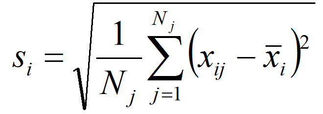
For a spatiotemporal variable composed of j time series observations at each of i locations, the standard deviation of anomalies at each location i is:
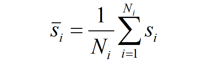
The mean anomaly standard deviation over all i locations is:
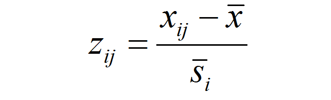
Each observation xij is spatiotemporally standardized to a unitless score zij by subtracting the grand mean of the variable, and dividing by the mean anomaly standard deviation:
Effect of spatio-temporal standardization on PCA feature extraction
In previous blog posts I found that PCA of globally standardized climate data was problematic because it allowed variables with large interannual (within-group) variability to dominate the climate space, even if there was relatively little spatial (between-group) variability. This was exemplified in climate space of south-central BC, where variables associated with winter temperatures (TD and MCMT) dominated the second principal component. This type of high within-group and low between-group variability is unlikely to be ecologically important, because organismal life strategies are adapted to it (e.g. via dormancy in plants). Discriminant analysis is designed to address this problematic type of variability, but I found that it goes too far: LDA extracts features only on the basis of the ratio of between- to within-group variability, regardless of whether those features are important to the overall spatiotemporal variability of the study area. A compromise between PCA and LDA is required.
Spatio-temporal standardization provides an effective approach to balancing within-group and between-group variability in feature extraction. By standardizing on average temporal variability of the study area, climate elements are given equal emphasis relative to each other at any given location. This is ecologically justified, since organismal life strategies can be expected to be adapted to the general scale of variability in each climate element at any given location. A PCA of spatiotemporally standardized data will then emphasize climate elements with high spatial variability.

Figure 1: biplots of the first two principal components of globally standardized and spatiotemporally standardized climate data for the BEC variants of south-central interior British Columbia (BG, PP, IDF, ICH, SBS, SBPS, MS, and ESSF BEC zones). Red arrows indicate correlations between the two PCs and the 14 standardized climate variables.
The difference between PCA on globally standardized and spatiotemporally standardized data is illustrated in biplots of reduced climate spaces for south-central interior BC (Figure 1). Winter temperature variables TD and MCMT dominate PC2 in the globally standardized data because of their high within-group variability. Spatiotemporal standardization leads to much better differentiation of BEC variants in PC2. Variability structure plots (Figure 2) indicate that the winter temperature feature is shifted from PC2 in the globally standardized data to PC4 in the spatiotemporally standardized data.

Figure 2: structure of variability in principal components of globally standardized and spatiotemporally standardized climate data for the BEC variants of south-central interior British Columbia (BG, PP, IDF, ICH, SBS, SBPS, MS, and ESSF BEC zones).
Effect of spatio-temporal standardization on climate-year classification
Spatio-temporal standardization performs centering and scaling by coefficients that are common to all observations of any given variable. Nevertheless, the relative scaling of the variables changes, which changes the relative importance of the variables in contributing to Euclidian distance measures. spatiotemporal standardization uses a denominator of temporal (within-group) variability. As a result, Euclidian metrics of spatiotemporally standardized data will emphasize variables with a high spatial (between-group) variation relative to temporal variation. As a result, it is logical that spatio-temporal standardization will improve nearest-neighbour classification. This effect is demonstrated in climate year classifications of BEC variants on globally vs. spatiotemporally standardized data (Figure 3). In this example, spatiotemporal standardization increases nearest-neighbour climate year differentiation from 36% to 41%. However, spatiotemporal standardization has no effect on LDA or QDA classification, since these methods include standardization procedures that override the a priori scaling of the input data.
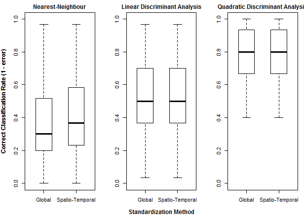
Figure 3: comparison of climate year classification rates for globally and spatiotemporally standardized data.
References
Williams, J. W., S. T. Jackson, and J. E. Kutzbach. 2007. Projected distributions of novel and disappearing climates by 2100 AD. Proceedings of the National Academy of Sciences of the United States of America 104:5738–42.
I am using per-pixel z-scores to compare differences in baseline and future climate means, as well as Williams SED method to aggregate z-scores into one metric of overall climate exposure for a region. But I can’t help but wonder: if the climate data is non-normally distributed are the z-scores meaningless? How does one account for this? There is a large body of literature that argues against the use of parametric statistics for analysis of climate data due to the issue of non-normality.
Hi Stephanie, apologies for the late response. i agree that z-scores aren’t meaningful for non-normal data. however, temporal climate variability at appropriate scales (e.g. controlled for diurnal and annual cycles) is often normally distributed or transformable to normal. Z-scores of temporal variability within any given pixel can be a good measure of dissimilarity, and there is a long tradition of using standardized anomalies this way within the atmospheric sciences (D. Wilks, statistical methods in the atmospheric sciences, is a good text). Perhaps the objections you are referring to are to z-scores of spatial (instead of temporal) variation in climate. the processes underlying spatial variation in climate should be expected to be non-normal. in addition, the meaning of a spatial z-score depends on the arbitrarily defined scale of the study area, which is not generally ecologically meaningful. I think that if you are using z-scores of temporal variation, and checking/transforming for univariate temporal normality, then there would be nothing wrong with your approach. i’m interested if you have further thoughts on this or reading suggestions.
Hi Colin,
Is this spatio-temporal standardisation equivalent to first spatially standardising the data, i.e. subtracting the mean of each pattern from the data, and then dividing the patterns by their standard deviations?
This approach has been used for map typing in Europe (cost733class-1.2 User Guide).
I would like to know your idea and discuss it with you.
Tayeb