Summary

In this post, PCA climate spaces are built from interannual climatic variability at centroid surrogates instead of spatial variability of climate normals. I found that patterns of spatial variability dominate the climate space because the spatial variation at the regional or provincial scale is much greater than the scale of interannual climatic variability at individual centroid surrogates. The conservation of spatial variation has the advantage that both spatial and temporal variability are represented in the reduced climate space. However, it has the disadvantage that temporal variability is inefficiently compiled into the principal components. I’m not sure of which method will help to address this issue. Another problem specific to PCA is that large variability in winter temperature causes related variables high weight in the PCs, even though there is little spatial variation in winter temperatures. This problem can be solved using LDA. Finally this post introduces the use of standard deviation of z-scores as a multivariate measure of interannual climatic variability.

Next steps are to experiment with discriminant analysis for this same purpose, and expand the analysis to assessment of climatic differentiation between BEC variants.

Introduction

To this point, I have been building multivariate climate spaces using spatial variation in climate normals. In this post, I take my first steps into climate spaces built from interannual climatic variability. The multivariate data set for this analysis is the annual climate elements at each BEC variant centroid surrogate for individual years in the 1961-1990 period. For conceptual simplicity, I use PCA for this stage of exploratory analysis.

Results

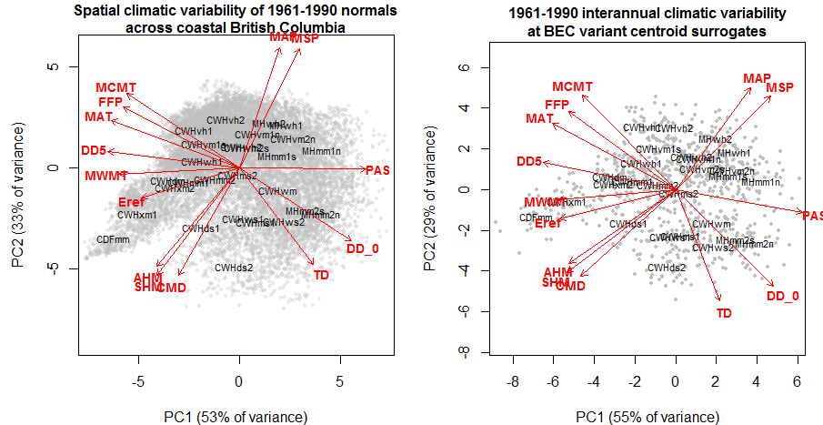
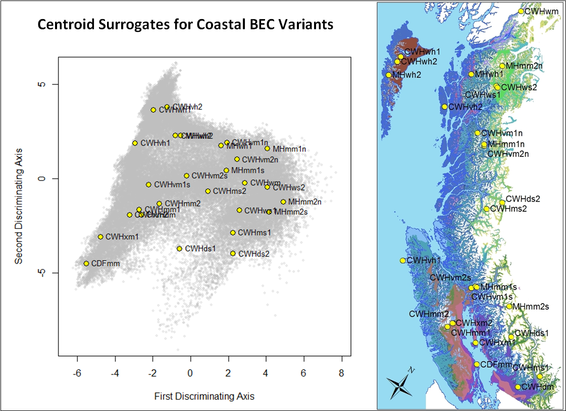
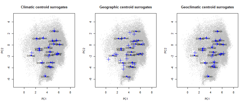
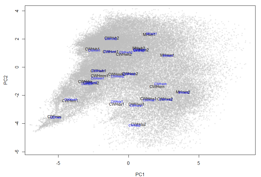
Figure 1: comparison of PCA rendering of spatial variability of climate normals at 1600-m grid points vs. interannual variability at BEC variant centroid surrogates. Data are for the characteristic BEC zones of coastal BC (CWH, CDF, MH).

The pattern of spatial climatic variation across the BC coast in is remarkably well preserved in the climate space of interannual variability at centroid surrogates (Figure 1). This indicates that interannual variability on the coast is of a lesser scale than the main spatial gradients in climate described by BEC variants.  The pattern of spatial variability is marginally less conserved in south and central interior BC (Figure 2). Notably, TD (the total difference between mean coldest and warmest month temperatures) is a very minor element in the spatial climate space, but is the primary correlate of PC2 in the temporal climate space. This is consistent with my previous result that there is very large interannual variability of winter temperatures in the BC interior, but little spatial variability in normals of winter temperature. The prominence of winter variability in the temporal climate space is likely undesirable for most purposes because it overrides other dimensions of variability that are much more important for differentiating BEC variants. This effect is also evident at the provincial scale (Figure 3), though it is more subtle due to the importance of TD in differentiating the coast from the interior of BC. Discriminant analysis may help to address this problem, especially at the regional scale, because it prioritizes climate elements that differentiate BEC variant centroid surrogates.

Figure 2: comparison of PCA rendering of spatial variability of climate normals at 1600-m grid points vs. interannual variability at BEC variant centroid surrogates. Data are for the characteristic BEC zones of South-central BC.

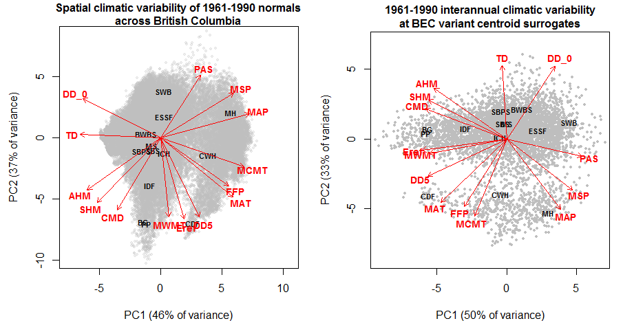
Figure 3: comparison of PCA rendering of spatial variability of climate normals at 1600-m grid points vs. interannual variability at centroid surrogates. Data are for the entire area of BC excluding alpine and subalpine parkland climates.

The graphs above demonstrate that, for the most part, the first two principal components are driven by spatial variation in average climatic conditions, even in the temporal data set. This is an inevitable result of the spatial variance at the regional and provincial levels being considerably greater than the temporal variance at individual points on the landscape.   The next question is: if spatial variation is overriding temporal variation in the PCA, how well do principal components of the temporal data set represent the important dimensions of interannual variability at each centroid surrogate?

Figure 4 demonstrates that there is a decreasing trend in the interannual variability of principal components. However, the decrease is much more gradual for the overall variance of the data set. On average it takes 7 of the 14 PCs to explain 95% of the variance in the climate years at individual centroid surrogates. Notably, the first three principal components are all equally important to describing interannual variability (25%, 22%, and 22% respectively, on average). These results indicate that PCA does not create an efficient reduced climate space for representing local interannual climatic variability.

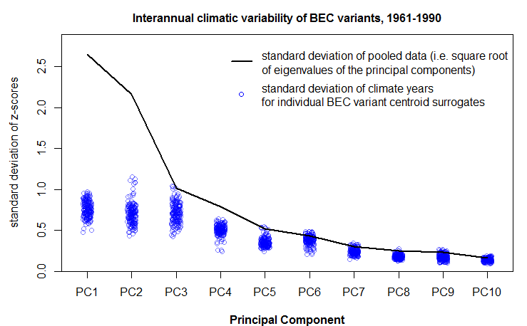
Figure 4: modified scree plot showing the total variability (in standard deviations) of each principal component, and the scale of interannual variability around each of the BEC variant centroid surrogates.

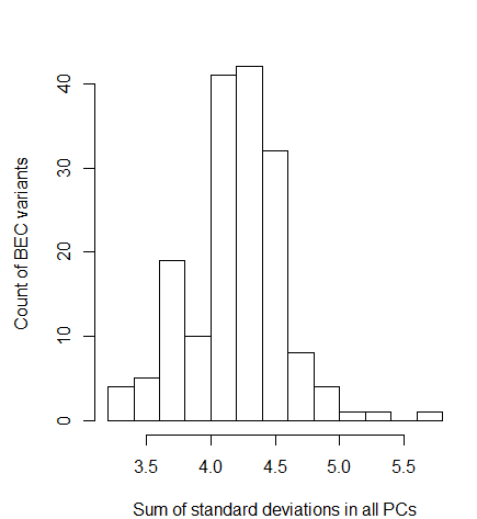
Figure 5: histogram of overall interannual climatic variability of BEC variant subzone surrogates.

Despite the potential inefficiencies of PCA as a dimension reduction tool, the graph above illustrates how standard deviation of z-scores can be used as a measure of interannual variability at each BEC variant centroid surrogate. There is reasonable variation between BEC variants in terms of this measure of interannual climatic variability (Figure 5). This variation facilitates mapping of overall climatic variability. Since the values of the map are total standard deviation across all PCs, they are a quantity of the raw data and are independent of any rotation.

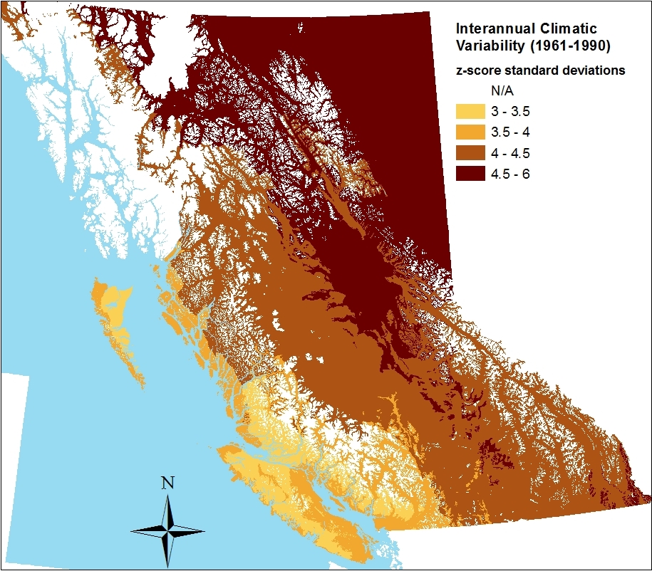
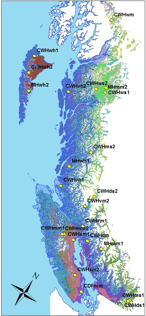
Figure 6: map of interannual climatic variability measured as the sum of standard deviations of z-scores in all principal components for each BEC variant centroid surrogate.

My analysis up to this point has used spatial variation in climate normals at 1600-m grid points. Time series analysis on the full 1600-m grid is impractical because each point would have a set of climate observations for each year over the period of the time series. This creates a lot of data, and a lot of redundant variation. An alternate approach is to use the BEC variants to define the ecologically appropriate scale of climate differentiation, and then use the climatic centroid of each BEC variant for time series analysis. The easiest way to do this is to find the 1600-m grid point whose climatic attributes are closest to the actual climatic centroid of the variant. I call this spatial location the climatic “centroid surrogate” for the BEC variant.

Mahalanobis distance vs Standardized Euclidian Distance

To find the “closest” grid point to the climatic centroid, one first has to select a distance measure. Simple Euclidian distance is not appropriate since climate elements have different units (e.g. ^oC vs. mm) and variables with large variance will dominate the distance measurement. The most straightforward approach is to standardize all the variables by subtracting the mean from each observation and dividing by the standard deviation. This converts all variables to units of standard deviation and a mean of zero, and facilitates a balanced measure of Euclidean distance. Another approach is to use Mahalanobis distance which also accounts for the correlation between variables. however, in practice I found mahalanobis distance to be difficult to implement in climate space due to the high collinearity between variables. For the purpose of finding a climatic centroid surrogate, standardized Euclidian distance and mahalanobis distance are likely to be equivalent. For this reason, I used standardized Euclidian distance.

Visual validation in climate space and map space

Figure 1: PCA climate space for the BC coast. BEC variants are labeled at their 2D pseudocentroids in black and full-dimensional (12D) centroid surrogates in blue. The close proximity of the labels provides visual validation that the centroid surrogate is at the climatic centroid.

Figure 2: locations of the climatic centroid surrogate for each coastal BEC variant.

The centroid surrogates are located very close to the BEC variant pseudocentroids of a two-dimensional PCA climate space representing 91% of the variance in the data (Figure 1). This strongly suggests that the calculation was correct and the centroid surrogate is the grid point with minimum distance to the climatic centroid. A map of the centroid surrogates (Figure 2) indicates that they are generally located in representative locations. However, there are several idiosyncrasies:

1. The centroid surrogate for the MHmm2 is located near Terrace in the northern portion of the variant’s geographic range, which extends all the way down to the U.S. border. This is problematic, since historical climate variability is likely to be different in the northern and southern areas of the MHmm2. Climate change forecasts are certainly very different for these two regions. This result suggests that more than one centroid surrogate may be required for variants with large geographic ranges (e.g. CWHvm1, vm2, MHmm1).
2. The centroid surrogate for the CWHwh1 is located in the mapped range of the CWHvh2. This is simply the result of using the BEC7 variant map for classification of the 1600-m grid points and the BEC8 map for mapping. This error will be corrected.
   

   Figure 3: close-up of the centroid surrogate for the CWHdm. It is located on the upper elevation limit of the CWHdm on East Redonda Island. While this location may represent the average climate of the CWHdm, it is not located in a core area of the variant. This result suggests the centroid surrogate selection method needs refinement.

3. The centroid surrogate for the CWHdm is located at the upper elevation limit of this variant’s occurrence on East Redonda Island (Figure 3). Intuitively, centroid surrogates should be located at approximately the geographic core of the BEC variant, rather than in transition zones. I attempted to prevent this problem by restricting centroid surrogate selection to grid points that are within one-half of a standard deviation of the mean elevation of each BEC variant. However, the same grid point was selected for the CWHdm, and resulted in poorer centroid surrogates for for submontane variants. As a result, the original solution shown in Figure 2 will be used for now. the potential for this issue should be kept in mind for other regions of the province as well.

Conclusion

The selection of centroid surrogates highlighted the important point that climatic zones that are considered now to represent relatively uniform climatic conditions may not have divergent historical and future variability. While centroid surrogates are useful for examining climatic differentiation in current conditions, they are not sufficient by themselves for characterizing climate change in BEC variants. Geographically extensive BEC variants likely need to have several centroid surrogates representing different regions of their distribution.