The distribution of precipitation in both space and time is typically skewed to the right. Since precipitation data cannot be expected to be normally distributed, the concept of variance has limited meaning for raw precipitation data. This raises the question of whether it is valid to use raw precipitation data within a principal components analysis (PCA), which is a variance-based technique. In this note, I evaluate this problem from both a statistical and ecological perspective.
The statistical rationale for transformation of precipitation variables towards a normal distribution prior to PCA is to facilitate a meaningful quantification of variance, and to stabilize the variance (reduce heteroskadacity). The ecological rationale for transformation of precipitation is that the meaning of the units changes across the range of values. For example, the ecological effect of a 100mm difference in annual precipitation is very different if the reference climate is 200mm vs 2000mm. Failing to transform precipitation variables may have profound implications for principal components analysis, because ecologically important variation at small precipitation values will be under-emphasized relative to ecologically less relevant variation at large values.
I have been surprised by the ambiguity surrounding whether or not data normality is an assumption of PCA. However, the predominant textbooks on PCA generally (Jolliffe 2002) and in the atmospheric sciences specifically (Wilks 2006) argue that PCA does not require multivariate normality of the data except for calculating inferential statistics on the PCs. Many sources informally state that normality is a “nice-to-have” for PCA, without explaining the implications of non-normal input data. Transformation of variables towards symmetric or normal distributions prior to PCA is a common practice (e.g. Wold et al. 1987, Baxter 1995) especially with regards to precipitation (e.g. Comrie and Glenn 1998, Hamann and Wang 2006).
Both Jolliffe (2002) and Wilks (2006) emphasize the critical importance of scaling the input variables so that their variance relative to each other is meaningful. It seems logical that this consideration could be applied to ensuring that the meaning of the data units is consistent throughout the range of the data in any given variable. The distribution of the data affects the direction (eigenvectors) and magnitude/rank (eigenvalues) of the principal components. Hence the distribution of each variable should be meaningful in the context of linear analysis. As mentioned previously, the ecological meaning of the raw units of precipitation (e.g. mm) depends on the reference condition (e.g. 200 vs. 2000 mm). a power transformation (e.g. log-transformation) is widely recommended to make the units of precipitation scale-dependent (e.g. Wilks 2006).
This post explores the effect of transformation on PCA using an example data set.
Methods
The data for this analysis is 1951-2000 climate normals compiled from CRU TS3.21 gridded data (Harris et al. 2013) for North America (Figure 1). I’ve also created 6 regional subsets of the data to help with interpretation of the graphs. Monthly temperature and precipitation were converted to the 19 Bioclim variables using the biovars {dismo} call in R.
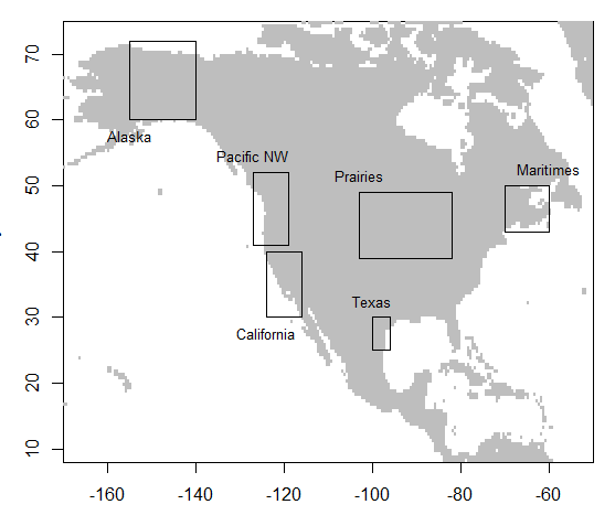
Figure 1: Extent of the North American study area used in this analysis, including the extents of the regional subsets.
Results
The distributions of 1951-2000 precipitation normals across North America are heavily skewed to the right (Figure 2). Log-transformation renders the distributions approximately symmetrical, though residual skewness in variables 14, 17, and 18 indicates that these variables are not log-normal and that adjusting the power transformation would be required to achieve symmetry.
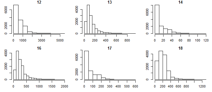
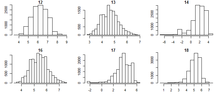
Figure 2: histograms of raw and log-transformed Bioclim precipitation normals for the north American study area. (BIO12 = Annual Precipitation; BIO13 = Precipitation of Wettest Month; BIO14 = Precipitation of Driest Month; BIO16 = Precipitation of Wettest Quarter; BIO17 = Precipitation of Driest Quarter; BIO18 = Precipitation of Warmest Quarter).
The effect of the skewness on the relationship between precipitation and temperature is illustrated in Figure 3. In the absence of transformation, the dispersion of the data is dominated by wetter climates. Log-transformation provides much greater resolution of the differences between moderate, dry, and very dry climates. However, it is not clear whether the principal component of this relationship would be substantially different in either data set.
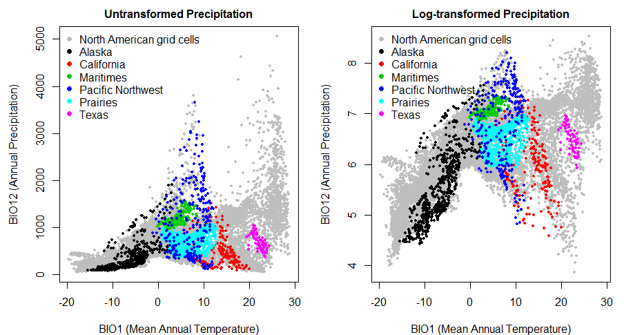
Figure 3: scatterplots of raw and log-transformed annual precipitation against mean annual temperature across North America.
PCA on the full set of 19 variables (Figure 4) suggests that transformation doesn’t have a major effect on the first two principal components: the differences between the correlations with the raw variables (red arrows) are only subtle in the two plots. However, scree plots (Figure 5) indicate that regional variance is partitioned quite differently in the two analyses, suggesting that there may be important differences in the third through sixth principal components.
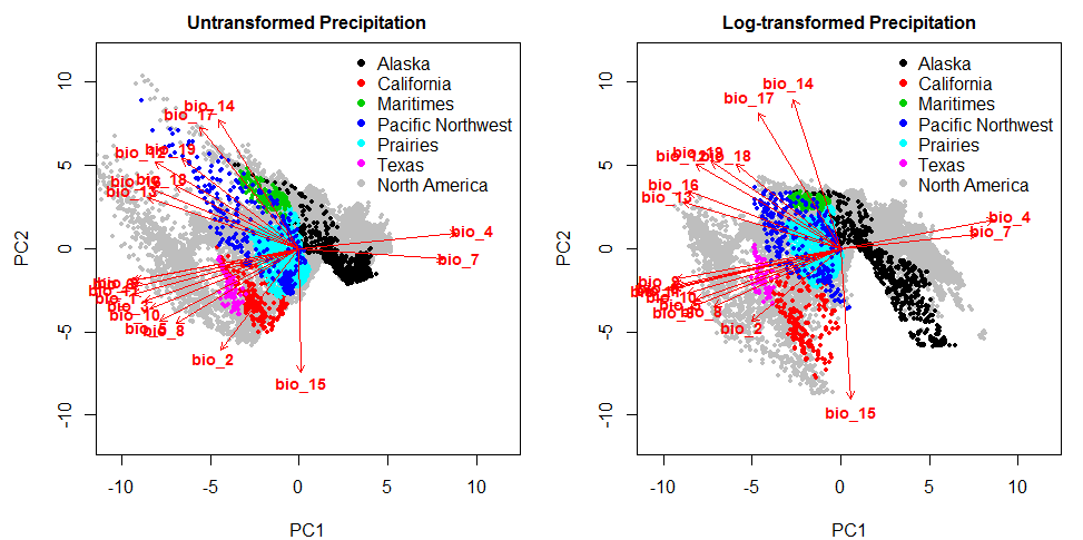
Figure 4: two-dimensional climate space of North America, showing correlation vectors with the BioClim variables (left) and the subspaces occupied by the regional subsets of the data.
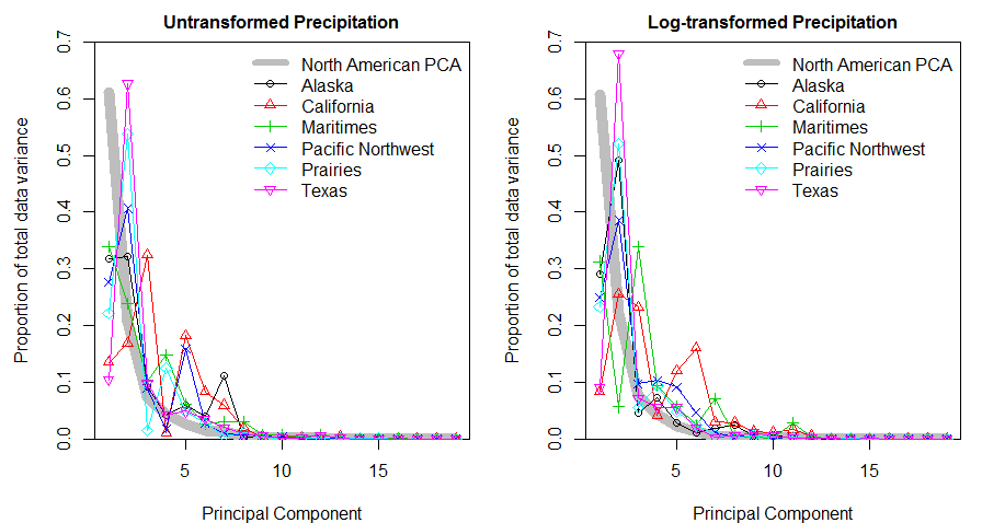
Figure 5: Scree plots of the North American PCA using raw and log-transformed precipitation, showing the proportion of total variation explained by each PC for the whole continental data set (grey line) and for regional subsets of the data.
Conclusions
It seems to be generally accepted that normality of input variables is not an assumption of PCA, unless inferential statistics are to be derived from the principal components. However, precipitation variables typically follow a heavily skewed gamma distribution, and transformation towards a normal distribution is a common practice to provide a more meaningful description of the data from both a statistical and ecological perspective. It is expected that transformation will influence the direction and magnitude of the principal components. However, the results of this case study indicated that the effect of transformation on the PCA was only subtle. There doesn’t appear to be an unequivocal requirement for transformation of precipitation data prior to PCA if subsequent analyses of the principal components do not require normality. Nevertheless, transforming precipitation data towards normality prior to PCA is highly recommended as a best practice.
References
Baxter, M. J. 1995. Standardization and Transformation in Principal Component Analysis, with Applications to Archaeometry. Journal of the Royal Statistical Society 44:513–527.
Comrie, A. C., and E. C. Glenn. 1998. Principal components-based regionalization of precipitation regimes across the southwest United States and northern Mexico , with an application to monsoon precipitation variability. Climate Research 10:201–215.
Hamann, A., and T. Wang. 2006. Potential Effects of Climate Change on Ecosystem and Tree Species Distribution in British Columbia. Ecology 87:2773–2786.
Harris, I., P. D. Jones, T. J. Osborn, and D. H. Lister. 2013. Updated high-resolution grids of monthly climatic observations – the CRU TS3.10 dataset. International Journal of Climatology 34:623–642.
Jolliffe, I. T. 2002. Principal Component Analysis, Second Edition. Page 487. Springer, New York.
Wilks, D. S. 2006. Statistical Methods in the Atmospheric Sciences, Second Edition. Page 627. Internatio. Academic Press.
Wold, S., K. Esbensen, and P. Geladi. 1987. Principal component analysis. Chemometrics and Intelligent Laboratory Systems 2:37–52.
Excerpts from the literature
Jolliffe (2002):
We digress slightly here to note that some authors imply, or even state explicitly, as do Qian et al. (1994), that PCA needs multivariate normality. This text takes a very different view and considers PCA as a mainly descriptive technique. It will become apparent that many of the properties and applications of PCA and related techniques described in later chapters, as well as the properties discussed in the present chapter, have no need for explicit distributional assumptions. It cannot be disputed that linearity and covariances/correlations, both of which play a central role in PCA, have especial relevance when distributions are multivariate normal, but this does not detract from the usefulness of PCA when data have other forms.
The distributional results outlined in the previous section may be used to make inferences about population PCs, given the sample PCs, provided that the necessary assumptions are valid. The major assumption that x has a multivariate normal distribution is often not satisfied and the practical value of the results is therefore limited. It can be argued that PCA should only ever be done for data that are, at least approximately, multivariate normal, for it is only then that ‘proper’ inferences can be made regarding the underlying population PCs. As already noted in Section 2.2, this is a rather narrow view of what PCA can do, as it is a much more widely applicable tool whose main use is descriptive rather than inferential. It can provide valuable descriptive information for a wide variety of data, whether the variables are continuous and normally distributed or not. The majority of applications of PCA successfully treat the technique as a purely descriptive tool, although Mandel (1972) argued that retaining m PCs in an analysis implicitly assumes a model for the data
Wilks (2006):
The distribution of the data x whose sample covariance matrix [S] is used to calculate a PCA need not be multivariate normal in order for the PCA to be valid. Regardless of the joint distribution of x, the resulting principal components ‘um will uniquely be those uncorrelated linear combinations that successively maximize the represented fractions of the variances on the diagonal of [S].
Comrie and Glenn (1998):
Pearson’s correlation coefficient used in the PCA input matrix can be sensitive to non-normality (White et al. 1991). In practice, PCA seems quite robust to moderate departures from normality of input data, but given the unusual precipitation distributions in some parts of the study area (especially stations with many zero precipitation months in the record), it seemed prudent to evaluate the regionalization using data transformed somewhat closer to normal. We examined frequency distributions across stations and experimented with several transformations, including the gamma distribution that is bounded on the left by zero and positively skewed, and therefore used in some precipitation studies. However, a simple square root transformation of monthly precipitation (p) appeared most useful when considered across all stations (i.e. p0.5).
Baxter (1995):
The logarithmic transformation, to base 10, of data before a principal component or other analysis is common. One reason for this is a belief that, within the raw materials of manufacture, elements have a natural log-normal distribution, and that normality of the data is desirable. A second reason is that a logarithmic transformation tends to stabilize the variance of the variables and would thus give them approximately equal weight in an unstandardized principal component analysis. A third reason sometimes cited is that, empirically, the use of a logarithmic transformation leads to more satisfactory results. In advocating the use of logarithmic transformation early work at the Brookhaven Laboratory has been influential (Bieber et al., 1976; Harbottle, 1976). Not everyone has been persuaded and a discussion of the issues involved and debate, with references, was given by Pollard (1986).
Wold et al. (1987):
Second, the data matrix can be subjected to transformations that make the data more symmetrically distributed, such as a logarithmic transformation, which was used in the swedes example above. Taking the logarithm of positively skewed data makes the tail of the data distribution shrink, often making the data more centrally distributed. This is commonly done with chromatographic data and trace element concentration data.
Thank you for this informative article. It provides a clear and thorough exploration of the considerations surrounding the use of raw precipitation data in principal components analysis (PCA). Your examination of both statistical and ecological rationales for data transformation, along with the practical results from your case study, offers valuable insights for researchers working with climate data. It reinforces the importance of carefully assessing data distribution and considering transformation as a best practice in PCA, even if not strictly required. Your work contributes to a better understanding of the nuances in this field.
A thought-provoking discussion on whether to transform precipitation variables before PCA. The statistical and ecological perspectives make a compelling case for transformation, but your analysis suggests subtle effects. It’s a valuable insight into a complex issue!