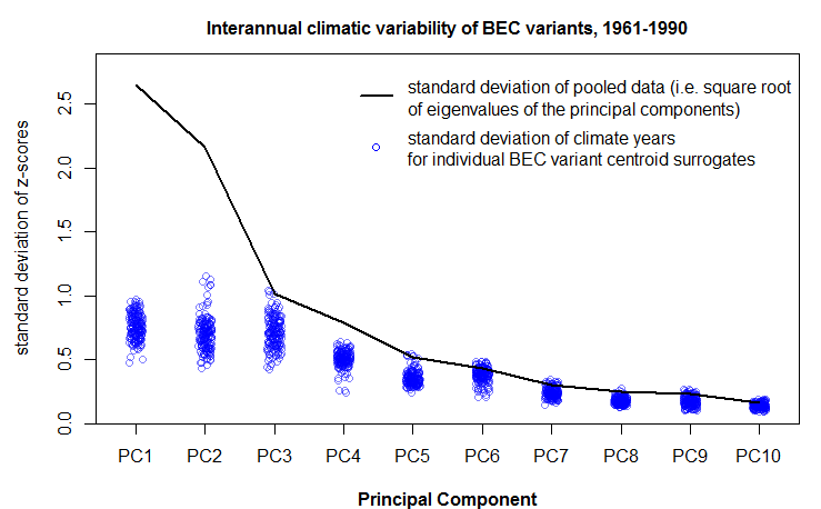
In the previous post I created a climate space using PCA on temporal climate variability at BEC variant centroid surrogates. This approach had the advantages of providing a climate space in which mahalanobis distance can be readily measured using Euclidian methods, and a metric—the z-score—which has direct meaning about the relative variability of the input variables. However, the PCA climate space gave too much emphasis to climate elements (e.g. TD, MCMT) with high temporal (within-group) variability but low spatial (between-group) variability. For most applications, that type of variability is not very ecologically meaningful. LDA is designed to emphasize variables with high ratios of between-group to within-group variance, so LDA can potentially create a more suitable climate space. LDA has the additional advantage of providing an analysis of classification error rate, which translates nicely into a climate year classification, i.e. what proportion of years are outside the “home” domain of each BEC variant. So my next step was to test run LDA on the data set of temporal climate variability at BEC variant centroid surrogates.
I replicated the analysis of the previous post, using LDA instead of PCA. Specifically, I used the lda() function of the MASS package in R. The most striking difference between the PCA and the LDA is that the LDA produces a climate space in which the within-groups variation is approximately equal to one in all dimensions (Figure 1). In contrast, the PCA produced a climate space in which the within-groups variation reflected the scale of variability in the raw data. The LDA result is highly problematic, because it obscures the structure of interannual climatic variability in the data. This result is due to a normalization procedure carried out in the lda() call: the R help file specifies that the scaling matrix (discriminating coefficients) is “normalized so that within groups covariance matrix is spherical.” This procedure is hard-wired into the call, and I couldn’t figure out how to reverse the normalization in the d-scores.
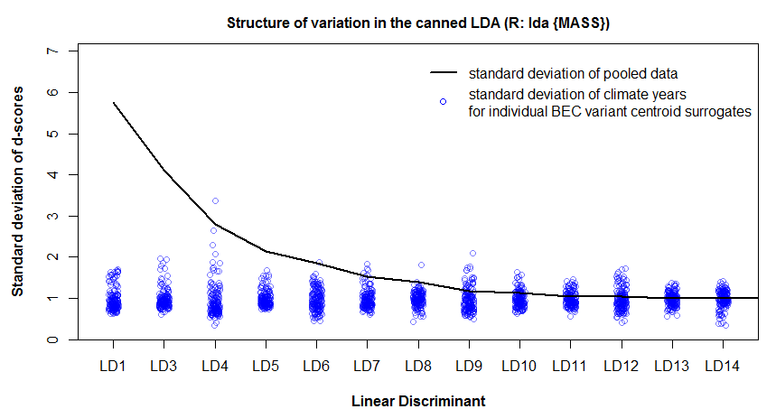
Figure 1: structure of total and within-group variation of discriminant scores resulting from a “canned” LDA using the “lda()” command from the {MASS} package of R. The mean within-group standard deviation is approximately equal to one due to normalization of the within-groups covariance matrix.
To produce an LDA without normalization of the within-groups covariance matrix (Sw), I did a “home-made” LDA in R based on a very clear explanation of first principles of LDA provided online by Dr. Ricardo Gutierrez-Osuna at Texas A&M University. My R code for this procedure is provided at the end of this post. The structure of variation is much more clear in the home-made LDA (Figure 2), and give an elegant illustration of how LDA extracts features with the highest ratio of between-groups to within groups variation. Note, for example, how LD6 is an axis of high variation: it has within-groups variation similar to LD1 and LD3, and total variation much greater than LD3 and LD4. It is lower in the order of LDs due to the ratio of between to within. LD4 in contrast, represents an axis of very low variation, but is prioritized because its between:within ratio is relatively large. For the purpose of classification, this structure is fine. However, for the purposes of dimension reduction this result is poor: LD4 and 5 should clearly not be prioritized over LD6 and 7. The structure of the PCA is likely preferable for dimension reduction.

Figure 2: structure of total and within-group variation of discriminant scores resulting from a “home-made” LDA that does not perform spherical normalization of the within-groups covariance matrix. The structure of climatic variation in the LDs is much more clear.

Figure 3: ratio of standard deviations of between- and within-group variation. This graph demonstrates the equivalence of this ratio with the eigenvalues of the linear discriminants.
How do these different methods compare in terms of classification? LDA classification is a nearest-neighbour classification of the data projected onto the linear discriminants. Based on this principle, I did a nearest-neighbour classification of the data in the full-dimensional (14D) PCA, LDA, and home-made LDA climate spaces. In this analysis, “correct” classification is the assignment of an observation to its own group. in other words, a climate year is “correctly” classified if it falls into the home domain (voronoi cell) of its own BEC variant. the correct classification rates of the PCA, home-made LDA, and canned LDA are 36%, 45%, and 53%, respectively (Figure 4). Clearly, Sw normalization is advantageous for classification. However, it is interesting that the classification error rates are so different. Given that all classifications were done on the full-dimensional data (14 extracted features from 14 raw variables), the classification effectiveness is not due to feature extraction in the sense of eigenvector selection. Instead, it appears that the differences in classification error rates are related to how the data are projected onto the extracted features. I will do some simulations to clarify this issue in the next post.
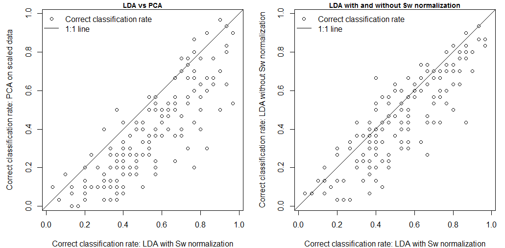
Figure 4: comparison of correct classification rates (climate years classified in their own BEC variants) for the PCA, the “canned” LDA with normalization of the within-groups covariance matrix (Sw), and the “home-made” LDA without Sw normalization.
Example R Code for “home-made” Linear Discriminant Analysis
# Linear Discriminant Analysis from first principles.
#development of method using 2-group, 2D discrim analysis
# following http://research.cs.tamu.edu/prism/lectures/pr/pr_l10.pdf
library(MASS) #contains the eqscplot(x,y) function, which plots axes of equal scale
x1 <- c(4,2,2,3,4,9,6,9,8,10)
x2 <- c(1,4,3,6,4,10,8,5,7,8)
X <- data.frame(x1,x2)
A <- c(1,1,1,1,1,2,2,2,2,2)
eqscplot(x1,x2,pch=A)
Ni <- table(A) #population size N for each group i
MUi <- aggregate(X,by=list(A),FUN=mean) #group mean vectors
MUi$Group.1 <- NULL
#within-groups Scatter matrices (covariance matrix for group i multiplied by group population size Ni)
Si <- list()
for(i in 1:length(levels(factor(A)))){
Si[[i]] <- var(X[which(as.numeric(A)==i),])*(Ni[i]-1)/Ni[i] #multiply by (N-1)/N because the var function calculates sample variance instead of population variance
}
#total within class scatter Sw (Matrix sum of the within-groups Scatter matrices)
SW <- Reduce(‘+’,Si)
dim(SW)
#between-groups scatter matrix (covariance matrix of the group means multiplied by group population size Ni)
SB <- var(MUi)*length(levels(factor(A)))
dim(SB)
#calculate the matrix ratio of between-groups to within-groups scatter (the command solve() provides the inverse of a square matrix)
J <- solve(SW)%*%SB
W.vec <- eigen(J)$vectors
W.val <- eigen(J)$values
# project the raw data onto the eigenvectors of J
Z<- as.matrix(X)%*%eigen(J)$vectors
Cor <- cor(X,Z) #correlations between LDs and Variables
##coordinates of grid points and pseudocentroids
x<- Z[,1]-mean(Z[,1])
y<- Z[,2]-mean(Z[,2])
xhat<-tapply(x, INDEX = A, FUN = mean, na.rm=TRUE)
yhat<-tapply(y, INDEX = A, FUN = mean, na.rm=TRUE)
###################### LD1xLD2 plot
eqscplot(x, y, pch = A, col = A, cex=1)
text(xhat,yhat, as.character(levels(factor(A))), col=”black”, cex=0.7, font=1) ##labels at the centroids
#add in Biplot arrows
EF <- 1 #arrow length modifier
arrows(0,0,Cor[,1]*EF*sd(x),Cor[,2]*EF*sd(x),len=0.1, col=”red”)
text(1.1*Cor[,1]*EF*sd(x),1.1*Cor[,2]*EF*sd(x), rownames(Cor), col=”red”, xpd=T, cex=0.9, font=2)